Книги+1 / 2013 [Chandan_Kumar_Sarkar]_Technology_CAD

E

X

L

1.43 eV

k

GaAs

Direct Band Gap Material

E

L

X

2.36 eV

k

AlAs

Indirect Band Gap Material

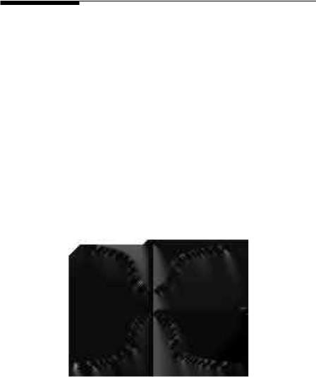
FIGURE 2.6

Energy band diagram in GaAs and AlAs.

material with a band gap of 1.43 eV. The direct (k = 0) conduction band minimum is denoted as λ. The lowest-lying indirect minimum is denoted as L and the other as X. In GaAs, as shown in Figure 2.6 (top), there are two higher-lying indirect minima, but these are sufficiently far above λ and few electrons reside there.

In AlAs shown in Figure 2.6 (bottom), the direct transition minimum is much higher than the indirect minimum and so this material is an example of indirect band-gap semiconductor with a band gap of 2.16 eV at room temperature. In the ternary compounds, all of these conduction band minima move up relative to the valence band, as the composition X varies from 0(GaAs) to 1(AlAs). However, the indirect minimum moves up less than the others when the compositions are above 38 percent Al. Also here this indirect minimum is actually the lowest-lying conduction band. AlGaAs is a direct band-gap semiconductor when X = 0 to X = 0.38 and is an indirect semiconductor for higher Al mole fractions. GaAs1–xPx is generally similar to AlGaAs, which is also a direct band-gap semiconductor up to X = 0.45. This material is

often used in light-emitting diode (LED) fabrication. Light emission is most efficient for direct materials, in which the electron can drop to the valence bands without changing k and therefore the momentum. By changing X, we can change the color of the light by changing the band gap [8].

2.3  Concept of Effective Mass

The effective mass of a semiconductor is obtained by fitting the actual E-k diagram around the conduction band minimum or the valence band maximum by a paraboloid shown in Figure 2.7. While this concept is simple enough, the issue turns out to be substantially more complex due to the occasional anisotropy of the minima and the maxima. A single electron is assumed to travel through a perfectly periodic lattice. The parameter m* called the effective mass takes into account all the internal forces in the lattice. Electrons are considered as classical particles whose motions are governed by classical mechanics when all the internal forces are taken care of through the concept of the effective mass.

Now classical laws like F = m*a are applied, where a is now directly related to external force. We know the electron momentum is p = mv = k, where the symbols have their usual significances. Thus,

E

k

FIGURE 2.7

Example of an E-K diagram.

2.4.1  Gauss’s Law

Gauss’s law gives a relationship between the charge density, ρ(x), and the electric field, E(x). Considering no time-dependent magnetic fields, the onedimensional equation is given by

Integrating the above equation, the electric field for 1D charge distribution is given as

In three dimensions, application of Gauss’s law gives the divergence of the electric field:

2.4.2  Poisson’s Equation

The electric field is defined as the negative gradient of the electrostatic potential, Ψ(x), or in one dimension, as the negative derivative of the electrostatic potential:

The electric field starts from a higher-potential region and points toward a lower-potential region.

Integration of the electric field gives the expression of potential as

Putting the expression of the electric field from Equation (2.8) into Equation (2.5), the relation between the charge density and the potential is obtained as

This equation is referred to as Poisson’s equation.

Combining Equations (2.11) and (2.7), the general form of Poisson’s equation is given by

2.4.3  Boltzmann Transport Equation

The Boltzmann transport equation (BTE) is a semi-classical approach to carrier transport. It describes the evolution of the trajectory of a particle by using a combination of Newtonian mechanics and quantum probabilistic scattering rates. The former account for the classical motion of the particle, and the latter for dissipative processes from one energy state to another. Unlike quantum transport, the energy eigen-states are not determined during the solution but are pre-computed by an independent method. The BTE can be derived from the Liouville-von Neumann transport equation under simplifying assumptions and ignoring all phase coherence [10,11]. A good introduction to the BTE, its physical parameters, and its application for device simulation can be found in [10].

For deriving the BTE a phase space is considered about the points (x, y, z, px, py, pz) as in [12], where (px, py, pz) are the angular components of p-type orbitals. The particles entering the considered phase space in time dt are equal to the number of

particles in (x − vxdt, y − vydt, z − vzdt, px − Fxdt, py − Fydt, pz − Fzdt) at some earlier dt time, where F is the external force on a particle and (Fx, Fy, Fz) are the respective

directional components of the force. Let the number of particles per unit volume in the phase space be represented by f(x, y, z, px, py, pz). The change in this distribution function in time dt as a result of the external force and the movement of particles is

given from [12] as df = f (x − vxdt, y − vydt, z − vzdt, px − Fxdt, py − Fydt, pz − Fzdt)

− f (x, y, z, px , py , pz ).

The time derivative of this function from Taylor series is given by dfdt = −(F p f + v r f ). However, if the scattering or collision of particles in the phase space due to particles from outside is considered, the time derivative takes the form

where ∂∂tf collision is the rate of change of distribution function due to collisions from other particles outside the phase space; s(r,p,t) is the term accounting

for the generation-recombination processes; s(r,p,t) stands for the probability

where tr is the transit time of carrier, moving with velocity, v, covering the distance L. The current density, J, can be expressed in terms of the charge density ρ as

Considering negatively charged electrons, the current density is given by

Considering positively charged holes, it is given by

where n and p are the semiconductor electron and hole density.

Due to scattering, the carriers move around the semiconductor randomly with a constantly changing path instead of a straight-line path along the electric field. This occurs when no electric field is applied externally and is due to the thermal carriers. Electrons in a non-degenerate electron gas have a thermal energy of kT/2 per particle per degree of freedom [1,19]. The typical thermal velocity is around 107 cm/s at room temperature, which is greater than the drift velocity in semiconductors. The movement of carriers in the semiconductor in the presence and absence of an electric field is shown in Figure 2.9.

When no external field is applied, the carriers move randomly with rapidly changing directions. On application of an external electric field, the holes move in the direction of the applied field, while the electrons move in the opposite direction.

The force on a carrier can be obtained from Newton’s law.

E = 0

x

FIGURE 2.9

Random motion of carriers in a semiconductor with and without an applied electric field.

The force equals the difference between the electrostatic force and the scattering force. The scattering force equals the ratio of the momentum of the carriers to the average time between collisions, τ—that is,

The average particle velocity can be obtained from Equation (2.21). In steady state, the carrier particles after acceleration reach a constant velocity. In such a condition, the velocity of the particle is proportional to the externally applied electric field. The mobility is defined as the average velocity per applied field.

Mobility of a semiconductor particle is small when the mass is large and the time between collisions is small. In terms of mobility, the drift current density for electrons may be expressed as

Similarly, the drift current density for holes may be expressed as

considering the mass, m, of the semiconductor particle. But the effective mass, m*, rather than the free particle mass, m, must be considered for taking into account the effect of the periodic potential of the atoms:

2.5.2  Diffusion Current

Semiconductor devices fall into two broad categories: majority carrier devices and minority carrier devices. In the majority carrier devices, current flow is dominated by electric fiield driven current. In minority carrier devices, the current flow is dominated by the diffusion effects. Whenever

there is a gradient in the concentration of mobile particles, the particles diffuse from the regions of high concentration to the regions of low concentration. In addition to drift, this is the alternate mechanism that can lead to current flow. Suppose a drop of ink falls into a glass of water. Introducing a high local concentration of ink molecules, the drop begins to “diffuse”—that is, the ink molecules tend to flow from a region of high concentration to regions of low concentration. This mechanism is called diffusion. A similar phenomenon occurs if charge carriers are dropped into a semiconductor so as to create a non-uniform density. In the absence of an electric field, the carriers move toward regions of low concentration, thereby carrying an electric current so long as the non-uniformity is sustained. Diffusion is therefore distinctly different from drift.

The derivation is based on the idea that carriers at non-zero temperature (Kelvin) have an additional thermal energy equal to kT/2 per degree of freedom. Thermal energy drives the diffusion process. At T = 0 K there is no diffusion. Because thermal energy is random, the average value needs to be considered for deriving the diffusion current for a one-dimensional semiconductor [1].

Let the average values of the thermal velocity be vth, the collision time τ, and the mean free path l. The thermal velocity is the average velocity of the semiconductor carriers in the positive or the negative direction. The collision time is the time taken by the carriers to move with the same velocity before a collision occurs with another carrier. The mean free path is the average length a carrier moves between collisions. From this basic concept the thermal velocity is given by

In order to find an expression for diffusion current density, a variable carrier density n(x) is considered in Figure 2.10. The carrier densities of two

n

n(–l)

n(+l)

FIGURE 2.10

Carrier density profile used to derive the diffusion current expression.