Confidence Interval Estimation

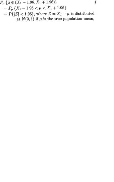
Next consider leading to the confi-

dence interval 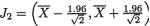. Let which is dis-

tributed as N(0, 1) if µ is the true population mean. Now, the confidence coefficient is given by

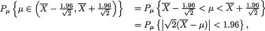
which is the same as P{| Z | < 1.96} = .95, whatever be µ. Between the two 95% confidence intervals J1 and J2 for µ, the interval J2 appears superior because J2 is shorter in length than J1. Observe that the construction of J2 is based on the sufficient statistic , the sample mean. !

In Section 9.2, we discuss some standard one–sample problems. The first approach discussed in Section 9.2.1 involves what is known as the inversion of a suitable test procedure. But, this approach becomes complicated particularly when two or more parameters are involved. A more flexible method is introduced in Section 9.2.2 by considering pivotal random variables. Next, we provide an interpretation of the confidence coefficient in Section 9.2.3. Then, in Section 9.2.4, we look into some notions of accuracy measures of confidence intervals. The Section 9.3 introduces a number of two–sample problems via pivotal approach. Simultaneous confidence regions are briefly addressed in Section 9.4.

It will become clear from this chapter that our focus lies in the methods of construction of exact confidence intervals. In discrete populations, for example binomial or Poisson, exact confidence interval procedures are often intractable. In such situations, one may derive useful approximate techniques assuming that the sample size is “large”. These topics fall in the realm of large sample inferences and hence their developments are delegated to the Chapter 12.

9.2One-Sample Problems

The first approach involves the inversion of a test procedure. Next, we provide a more flexible method using pivots which functionally depend only on the (minimal) sufficient statistics. Then, an interpretation is given for the confidence interval, followed by notions of accuracy measures associated with a confidence interval.

446 9. Confidence Interval Estimation

In other words, we can claim that

The equation (9.2.7) can be rewritten as

confidence interval estimator for θ. !

Example 9.2.3 (Example 9.2.2 Continued) Let X1, ..., Xn be iid with the common exponential pdf θ–1 exp{ –x/θ}I(x > 0) with the unknown parameter θ +. With preassigned α (0,1), suppose that we invert the UMP level α test for H0 : θ = θ0 versus H1 : θ < θ0, where θ0 is a positive real number.

Figure 9.2.3. The Area on the Left (or Right) of , 1– α Is a (or 1 – α)

dence interval estimator for θ, by inverting the UMP level α test. See the Figure 9.2.3. We leave out the details as an exercise. !

9.2.2The Pivotal Approach

Let X1, ..., Xn be iid real valued random variables from a population with the pmf or pdf f(x; θ) for x χ where θ( Θ) is an unknown real valued parameter. Suppose that T ≡ T(X) is a real valued (minimal) sufficient statistic for θ.

The family of pmf or pdf induced by the statistic T is denoted by g(t; θ) for t T and θ Θ. In many applications, g(t; θ) will belong to an appropriate location, scale, or location–scale family of distributions which were discussed in Section 6.5.1. We may expect the following results:

The Location Case: With some a(θ), the distribution of {T – a(θ)} would not involve θ for any θ Θ.

The Scale Case: With some b(θ), the distribution of

T/b(θ) would not involve θ for any θ Θ.

The Location–Scale Case: With some a(θ), b(θ), the distribution of {T – a(θ)}/b(θ) would not involve θ for any θ Θ.

Definition 9.2.1 A pivot is a random variable U which functionally depends on both the (minimal) sufficient statistic T and θ, but the distribution of U does not involve θ for any θ Θ.

In the location, scale, and location–scale situations, when U, T and θ are all real valued, the customary pivots are appropriate multiples of {T – a(θ)}, T/b(θ) or {T – a(θ)}/b(θ) respectively with suitable expressions of a(θ) and b(θ).

We often demand that the distribution of the pivot must coincide with one of the standard distributions so that a standard statistical table can be utilized to determine the appropriate percentiles of the distribution.

Example 9.2.4 Let X be a random variable with its pdf f(x; θ) = θ–1 exp{

–x/θ}I(x > 0) where θ(> 0) is the unknown parameter. Given some α (0,1), we wish to construct a (1 – α) two–sided confidence interval for θ. The statistic X is minimal sufficient for θ and the pdf of X belongs to the scale family. The pdf of the pivot U = X/θ is given by g(u) = e–uI(u > 0). One can explicitly determine two positive numbers a < b such that P(U < a) = P(U > b) = ½α so that P(a < U < b) = 1 – α. It can be easily checked that a = –log(1

– ½α) and b = –log(½α).

Since the distribution of U does not involve θ, we can determine both a and b depending exclusively upon α.

Now observe that

which shows that J = (b–1 X, a–1 X) is a (1 – α) two–sided confidence interval estimator for θ. !

448 9. Confidence Interval Estimation

Example 9.2.5 Let X1, ..., Xn be iid Uniform(0, θ) where θ(> 0) is the unknown parameter. Given some α (0,1), we wish to construct a (1 – α) two-sided confidence interval for θ. The statistic T ≡ Xn:n, the largest order statistic, is minimal sufficient for θ and the pdf of T belongs to the scale family. The pdf of the pivot U = T/θ is given by g(u) = nun–1I(0 < u <1). One can explicitly determine two numbers 0 < a < b < 1 such that P(U < a) = P(U > b) = ½α so that P(a < U < b) = 1 – α. It can be easily checked that a = (½α)1/n and b = (1 – ½α)1/n. Observe that

which shows that J = (b–1 Xn:n, a–1 Xn:n) is a (1 – α) two–sided confidence interval estimator for θ. !

Example 9.2.6 Negative Exponential Location Parameter with Known Scale: Let X1, ..., Xn be iid with the common negative exponential pdf f(x; θ) = σ–1 exp{–(x – θ)/σ}I(x > θ). Here, θ is the unknown parameter and we assume that σ + is known. Given some α (0,1), we wish to construct a (1 – α) two–sided confidence interval for θ. The statistic T ≡ Xn:1, the smallest order statistic, is minimal sufficient for θ and the pdf of T belongs to the location family. The pdf of the pivot U = n(T – θ)/σ is given by g(u) = e–uI(u > 0). One can explicitly determine a positive number b such that P(U > b) = a so that we will then have P(0 < U < b) = 1 – α. It can be easily checked that b = –log(α). Observe that

which shows that J = (Xn:1 – bn–1 σ, Xn:1) is a (1 – α) two-sided confidence interval estimator for θ.

Figure 9.2.4. Standard Normal PDF: The Area on the

Right (or Left) of zα/2 (or – zα/2) Is α/2

Example 9.2.7 Normal Mean with Known Variance: Let X1, ...,

Xn be iid N(µ, σ2) with the unknown parameter µ . We assume that

σ + is known. Given some α (0,1), we wish to construct a (1 – α) twosided confidence interval for µ. The statistic T = , the sample mean, is minimal sufficient for µ and T has the N(µ, 1/nσ2) distribution which belongs to the location family. The pivot U = has the standard normal distribution. See the Figure 9.2.4. We have P{ –zα/2 < U < zα/2} = 1 – α which implies that

In other words,

is a (1 – α) two–sided confidence interval estimator for µ. !

Example 9.2.8 Normal Mean with Unknown Variance: Suppose that

X1, ..., Xn are iid N(µ, α2) with both unknown parameters µ and σ+, n ≥ 2. Given some α (0,1), we wish to construct a (1 – α) twosided confidence interval for µ. Let be the sample mean and

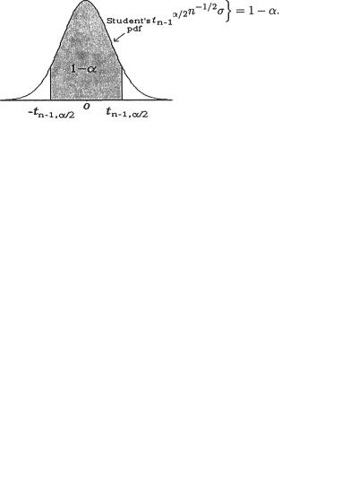
be the sample variance. The statistic T ≡ (, S) is minimal sufficient for (µ, σ). Here, the distributions of the X’s belong to the location–scale family. The pivot has the Student’s t distribution with (n – 1) degrees of freedom. So, we can say

that P{ –tn–1,α/2 < U < tn–1,α/2} = 1 – α where tn–1,α/2 is the upper 100(1 – ½α)% point of the Student’s t distribution with (n – 1) degrees of free-

dom. See the Figure 9.2.5.

Figure 9.2.5. The Area on the Right (or Left) of tn–1,α/2 (or –tn–1,α/2) Is α/2

Example 9.2.10 Joint Confidence Intervals for the Normal Mean and Variance: Suppose that X1, ..., Xn are iid N(µ, σ2) with both unknown parameters µ and σ +, n ≥ 2. Given some α (0, 1), we wish to construct (1 – α) joint two-sided confidence intervals for both µ and σ2. Let be the sample mean and be the sample variance. The statistic T ≡ (, S) is minimal sufficient for (µ, σ).

From the Example 9.2.8, we claim that

is a (1 – γ) confidence interval for µ for any fixed γ (0, 1). Similarly, from the Example 9.2.9, we claim that

is a (1 – δ) confidence interval for σ2 for any δ (0, 1). Now, we can write

Now, if we choose 0 < γ , δ < 1 so that γ + δ = α, then we can think of {J1, J2} as the two-sided joint confidence intervals for the unknown parameters µ, σ2 respectively with the joint confidence coefficient at least (1 – α). Customarily, we pick γ = δ = ½α. !

One will find more closely related problems on joint confidence intervals in the Exercise 9.2.7 and Exercises 9.2.11-9.2.12.

9.2.3The Interpretation of a Confidence Coefficient

Next, let us explain in general how we interpret the confidence coefficient or the coverage probability defined by (9.1.1). Consider the confidence interval J for θ. Once we observe a particular data X = x, a two-sided confidence interval estimate of θ is going to be (TL(x), TU(x)), a fixed subinterval of the real line. Note that there is nothing random about this observed interval estimate (TL(x), TU(x)) and recall that the parameter θ is unknown ( Θ) but it is a fixed entity. The interpretation of the phrase “(1 – α) confidence” simply means this: Suppose hypothetically that we keep observing different data X = x1, x2, x3, ... for a long time, and we

452 9. Confidence Interval Estimation

keep constructing the corresponding observed confidence interval estimates (TL(x1), TU(x1)), (TL(x2), TU(x2)), (TL(x3), TU(x3)), .... In the long run, out of all these intervals constructed, approximately 100(1 – α)% would include the unknown value of the parameter θ. This goes hand in hand with the relative frequency interpretation of probability calculations explained in Chapter 1.

In a frequentist paradigm, one does not talk about the probability of a fixed interval estimate including or not including the unknown value of θ.

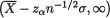
Example 9.2.11 (Example 9.2.1 Continued) Suppose that X1, ..., Xn are iid N(µ, σ2) with the unknown parameter µ . We assume that s &plus; is

known. We fix α = .05 so that will be a 95% lower

confidence interval for µ. Using the MINITAB Release 12.1, we generated a normal population with µ = 5 and σ = 1. First, we considered n = 10. In the ith replication, we obtained the value of the sample mean and computed the

lower end point of the observed confidence interval, i = 1, ..., k

with k = 100, 200, 500. Then, approximately 5% of the total number (k) of intervals so constructed can be expected not to include the true value µ = 5. Next, we repeated the simulated exercise when n = 20. The following table summarizes the findings.

Table 9.2.1. Number of Intervals Not Including the True Value

µ = 5 Out of k Simulated Confidence Intervals

The number of simulations (k) is not particularly very high in this example. Yet, we notice about four or five percent non–coverage which is what one may expect. Among k constructed intervals, if nk denotes the number of intervals which do not include the true value of µ, then we can claim that

9.2.4Ideas of Accuracy Measures

In the two Examples 9.2.7–9.2.8 we used the equal tail percentage points of the standard normal and the Student’s t distributions. Here, both pivotal distributions were symmetric about the origin. Both the standard normal and the Student’s tn–1 pdf’s obviously integrate to (1 – α) re-

spectively on the intervals (–zα/2,zα/2) and (–tn–1,α/2,tn–1,α/2). But, for these two distributions, if there existed any asymmetric (around zero) and shorter

interval with the same coverage probability (1 – α), then we should have instead mimicked that in order to arrive at the proposed confidence intervals.

Let us focus on the Example 9.2.7 and explain the case in point. Suppose that Z is the standard normal random variable. Now, we have P{–zα/2 < Z < zα/2} = 1 – α. Suppose that one can determine two other positive numbers a,

b such that P{–a < Z < b} = 1 – α and at the same time 2zα/2 > b + a. That is, the two intervals (–zα/2,zα/2) and (–a, b) have the same coverage probability

(1 – α), but (–a, b) is a shorter interval. In that case, instead of the solution

proposed in (9.2.9), we should have suggested 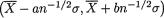as the confidence interval for µ. One may ask: Was the solution in (9.2.9) proposed because the interval (–zα/2,zα/2) happened to be the shortest one with (1 – α) coverage in a standard normal distribution? The answer is: yes, that is so. In the case of the Example 9.2.8, the situation is not quite the same but it remains similar. This will become clear if one contrasts the two Examples 9.2.12–9.2.13. For the record, let us prove the Theorem 9.2.1 first.

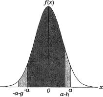
Figure 9.2.7. The Area Between –a and a Is (1 – θ). The Area Between –(a + g) and (a – h) Is (1 – θ)

Theorem 9.2.1 Suppose that X is a continuous random variable having a unimodal pdf f(x) with the support . Assume that f(x) is symmetric around x = 0, that is f(–x) = f(x) for all x > 0. Let P(–a < X < a) = 1 – a for some 0 < α < ½. Now, suppose that the positive numbers g, h are such that one has P(– a – g < X < a – h) = 1 – α. Then, the interval (–a – g, a – h) must be wider than the interval (–a, a).

Proof It will suffice to show that g > h. The mode of f(x) must be at

454 9. Confidence Interval Estimation

x = 0. We may assume that a > h since we have 0 < α < ½. Since we have P(–a < X < a) = P(–a – g < X < a – h), one obviously, has

But, the pdf f(x) is symmetric about x = 0 and f(x) is assumed positive for all x . The Figure 9.2.7 describes a situation like this. Hence, the integrals in

(9.2.15) can be equal if and only if 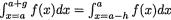which can

happen as long as the interval (a – h, a) is shorter than the interval (a, a +g). The result then follows. The details are left out as an exercise. !

Remark 9.2.1 The Theorem 9.2.1 proved that among all (1 – α) intervals going to the left of (–a, a), the interval (–a, a) was the shortest one. Since, f(x) is assumed symmetric about x = 0, it also follows from this result that among all (1 – α) intervals going to the right of (–a, a), the interval (–a, a) is again the shortest one.

Example 9.2.12 (Example 9.2.7 Continued) The length Ln of the confidence interval from (9.2.9) amounts to 2zα/2n–½σ which is the shortest width among all (1 – α) confidence intervals for the unknown mean µ in a N(µ, σ2) population with σ(> 0) known. The Theorem 9.2.1 immediately applies. Also observe that the shortest width, namely 2zα/2n–½σ, is a fixed number here.

Example 9.2.13 (Example 9.2.8 Continued) The length Ln of the confidence interval from (9.2.10) amounts to 2tn–1,α/2n–½S which is a random variable to begin with. So, we do not discuss whether the confidence interval from (9.2.10) has the shortest width among all (1 – α) confidence intervals for the unknown mean µ. The width Ln is not even a fixed number! Observe

rectly implies that the confidence interval from (9.2.10) has the shortest expected width among all (1 – a) confidence intervals for µ in a N(µ, s2) population when σ2(> 0) is also unknown. !

Both examples handled the location parameter estimation problems and we could claim the optimality properties (shortest width or shortest expected width) associated with the proposed (1 – α) confidence intervals. Since the pivotal pdf’s were symmetric about zero and unimodal, these intervals had each tail area probability ½α. Recall the Figures 9.2.4–9.2.5.

In the location parameter case, even if the pivotal pdf is skewed but unimodal, a suitable concept of “optimality” of (1 – α) confidence intervals can be formulated. The corresponding result will coincide with Theorem

9.2.1 in the symmetric case. But, any “optimality” property in the skewed unimodal case does not easily translate into something nice and simple under the scale parameter scenario. For skewed pivotal distributions, in general, we can not claim useful and attractive optimality properties when a (1 – α) confidence interval is constructed with the tail area probability ½α on both sides.

Convention: For standard pivotal distributions such as Normal, Student’s t, Chi–square and F, we customarily assign the tail area probability ½α on both sides in order to construct a 100(1 – α)% confidence interval.

9.2.5Using Confidence Intervals in the Tests of Hypothesis

Let us think of testing a null hypothesis H0 : θ = θ0 against an alternative hypothesis H1 : θ > θ0 (or H1 : θ < θ0 or H1 : θ ≠ θ0). Depending on the nature of the alternative hypothesis, the rejection region R respectively becomes upper or lower or two-sided. The reader has observed that a confidence interval for θ can also be upper or lower or two-sided.

Suppose that one has constructed a (1 – α) lower confidence interval estimator J1 = (TL(X), ∞) for θ. Then any null hypothesis H0 : θ = θ0 will be rejected at level α in favor of the alternative hypothesis H1 : θ > θ0 if and only if θ0 falls outside the confidence interval J1.

Suppose that one has constructed a (1 – α) upper confidence interval estimator J2 = (–∞, TU(X)) for θ. Then any null hypothesis H0 : θ = θ0 will be rejected at level α in favor of the alternative hypothesis H1 : θ < θ0 if and only if θ0 falls outside the confidence interval J2.

Suppose that one has constructed a (1 – α) two–sided confidence interval estimator J3 = (TL(X), TU(X)) for θ. Then any null hypothesis H0 : θ = θ0 will be rejected at level a in favor of the alternative hypothesis H1 : θ ≠ θ0 if and only if θ0 falls outside the confidence interval J3.

Once we have a (1 – α) confidence interval J, it is clear that any null hypothesis H0 : θ = θ0 will be rejected at level α as long as θ0 J. But, rejection of H0 leads to acceptance of H1 whose nature depends upon whether J is upper-, loweror two-sided.

Sample size determination is crucial in practice if we wish to have a preassigned “size” of a confidence region. See Chapter 13.

456 9. Confidence Interval Estimation

9.3Two-Sample Problems

Tests of hypotheses for the equality of means or variances of two independent populations need machineries which are different in flavor from the theory of MP or UMP tests developed in Chapter 8. These topics are delegated to Chapter 11. So, in order to construct confidence intervals for the difference of means (or location parameters) and the ratio of variances (or the scale parameters), we avoid approaching the problems through the inversion of test procedures. Instead, we focus only on the pivotal techniques.

Here, the basic principles remain same as in Section 9.2.2. For an unknown real valued parametric function κ(θ), suppose that we have a point estimator which is based on a (minimal) sufficient statistic T for θ. Often, the exact distribution of will become free from θ for all θ Θ with some τ(> 0).

If τ happens to be known, then we obtain two suitable numbers a and b

such that Pθ[a < { – κ(θ)}/τ < b] = 1 – α. This will lead to a (1 – α) twosided confidence interval for κ(θ).

If τ happens to be unknown, then we may estimate it by and use the new pivot instead. If the exact distribution of { – become free from θ for all θ Θ, then again we obtain two suitable numbers a and b such that Once more this will lead to a (1 – α) two-sided confidence interval for κ(θ). This is the way we will handle the location parameter cases.

In a scale parameter case, we may proceed with a pivot whose distribution will often remain the same for all θ Θ. Then, we obtain two suitable numbers a and b such that . This will lead to a (1 – α) two–sided confidence interval for κ(θ).

9.3.1Comparing the Location Parameters

Examples include estimation of the difference of (i) the means of two independent normal populations, (ii) the location parameters of two independent negative exponential populations, and (iii) the means of a bivariate normal population.

Example 9.3.1 Difference of Normal Means with a Common Unknown Variance: Recall the Example 4.5.2 as needed. Suppose that the

random variables Xi1, ..., Xin, are iid N(µi, σ2), i = 1, 2, and that the X1j’s are independent of the X2j’s. We assume that all three parameters are un-

known and θ = (µ1, µ2, σ) × × +. With fixed α (0, 1), we wish to construct a (1 – α) two–sided confidence interval for µ1 – µ2(= κ(θ))

based on the sufficient statistics for θ. With ni ≥ 2, let us denote

for i = 1, 2. Here, is the pooled sample variance.

Based on (4.5.8), we define the pivot

which has the Student’s tv distribution with v = (n1 + n2 – 2) degrees of

freedom. Now, we have P{–tv,α/2 < U < tv,α/2} = 1 – α where tv,α/2 is the upper 100(1 – ½α)% point of the Student’s t distribution with v degrees of free-

dom. Thus, we claim that

Now, writing , we have

as our (1 – α) two–sided confidence interval for µ1 – µ2. !

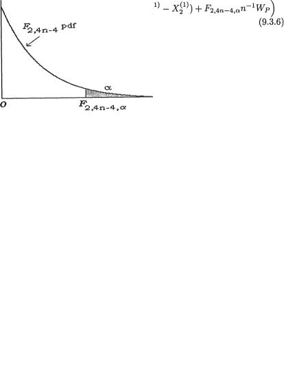
Example 9.3.2 Difference of Negative Exponential Locations with a Common Unknown Scale: Suppose that the random variables Xi1, ..., Xin are iid having the common pdf f(x; µi, σ), i = 1, 2, where we denote f(x; µ, σ) = σ–1 exp{ – (x – µ)/σ}I(x > µ). Also let the X1j’s be independent of the X2j’s. We assume that all three parameters are unknown and α = (µ1, µ2, σ)× × +. With fixed α (0, 1), we wish to construct a (1 – α) two–sided confidence interval for µ1 – µ2(= κ(α)) based on the sufficient statistics for α. With n ≥ 2, let us denote

for i = 1, 2.

Here, WP is the pooled estimator of σ. It is easy to verify that WP estimates σ unbiasedly too. It is also easy to verify the following claims:

That is, V[WP] < V[Wi], i = 1, 2 so that the pooled estimator WP is indeed a better unbiased estimator of s than either Wi, i = 1, 2.

Confidence interval estimation of (µ1 – µ2)/σ in the two Examples 9.3.1-9.3.2 using the Bonferroni inequality are left as Exercises 9.3.3 and 9.3.5. Look at the Example 9.2.10 as needed.

Example 9.3.3 The Paired Difference t Method: Sometimes the two populations may be assumed normal but they may be dependent. In a large establishment, for example, suppose that X1j, X2j respectively denote the job performance score before and after going through a week–long job enhancement program for the jth employee, j = 1, ..., n(≥ 2). We assume that these employees are selected randomly and independently of each other. We wish to compare the average “before and after” job performance scores in the population. Here, observe that X1j, X2j, are dependent random variables. The methodology from the Example 9.3.1 will not apply here.

Suppose that the pairs of random variables (X1j, X2j) are iid bivariate normal, 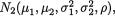j = 1, ..., n(≥ 2). Let all five parameters be unknown, (µi, σi) × +, i = 1, 2 and –1 < ρ < 1. With fixed α (0, 1), we wish to construct a (1 – α) two–sided confidence interval for µ1 – µ2 based on the sufficient statistics for θ ( = (µ1, µ2, σ1, σ2, ρ)). Let us denote

In (9.3.7), observe that Y1, ..., Yn are iid N(µ1 – µ2, σ2) where

Since both mean µ1 – µ2 and variance σ2 of the common normal distribution of the Y’s are unknown, the original two-sample problem reduces to a one–sample problem (Example 9.2.8) in terms of the random samples on the Y’s.

We consider the pivot

which has the Student’s t distribution with (n – 1) degrees of freedom. As

before, let tn–1,α/2 be the upper 100(1 – ½α)% point of the Student’s t distribution with (n – 1) degrees of freedom. Thus, along the lines of the Example

9.2.8, we propose

as our (1 – α) two–sided confidence interval estimator for (µ1 – µ2). !

460 9. Confidence Interval Estimation

9.3.2Comparing the Scale Parameters

The examples include estimation of the ratio of (i) the variances of two independent normal populations, (ii) the scale parameters of two independent negative exponential populations, and (iii) the scale parameters of two independent uniform populations.

Example 9.3.4 Ratio of Normal Variances: Recall the Example 4.5.3 as

needed. Suppose that the random variables Xi1, ..., Xini are iid ni ≥ 2, i = 1, 2, and that the X1j’s are independent of the X2j’s. We assume that all

four parameters are unknown and (µi, σi) × +, i = 1, 2. With fixed α (0, 1), we wish to construct a (1 – α) two-sided confidence interval for based on the sufficient statistics for θ(= (µ1, µ2, σ1, σ2)). Let us denote

for i = 1, 2 and consider the pivot

It should be clear that U is distributed as Fn1–1,n2–1 since (ni – 1) is distributed as i = 1, 2, and these are also independent. As before, let us

denote the upper 100(α/2)% point of the Fn1–1,n2–1 distribution by Fn1–1,n2–1,α/ 2. See the Figure 9.3.2.

Figure 9.3.2. Area on the Right (or Left) of Fn1–1,n2–1,α/2}

(or Fn1–1mn2–1,1–α/2) Is α/2

Thus, we can write P{Fn1–1,n2–1,1–α/2 < U Fn1–1,n2–1,α/2} = 1 – α and claim that

Hence, we conclude that

is a (1 – α) two-sided confidence interval estimator for the variance ratio By taking the square root throughout, it follows immediately from

(9.3.11) that

is a (1 – α) two–sided confidence interval estimator for the ratio σ1/σ2. !

Example 9.3.5 Ratio of Negative Exponential Scales: Suppose that

the random variables Xi1, ..., Xini are iid having the common pdf f(x; µi, si), ni ≥ 2, i = 1, 2, where f(x; µ, σ) = σ–1 exp{–(x – µ)/σ}I(x > µ). Also let the X1j’s be independent of the X2j’s. Here we assume that all four

parameters are unknown and (µi, σi) × +, i = 1, 2. With fixed α (0, 1), we wish to construct a (1 – α) two–sided confidence interval for σ1/ σ2 based on the sufficient statistics for θ ( = (µ1, µ2, σ1, σ2)). We denote

for i = 1, 2 and consider the pivot

It is clear that U is distributed as F2n1–2,2n2–2 since 2(nl – 1)Wl/σi is distributed as and these are also independent. As before, let us

denote the upper 100(α/2)% point of the F2n1–2,2n2 – 2 distribution by

Fn1–2,2n2–2,α/2. Thus, we can write P{F2n1–2,2n2–2,1–α/2 < U < F2n1–2,2n2–2,α/2} =

1 – α and hence claim that

462 9. Confidence Interval Estimation

This leads to the following conclusion:

is a (1 – α) two–sided confidence interval estimator for σ1/σ2. !

Example 9.3.6 Ratio of Uniform Scales: Suppose that the random variables Xi1, ..., Xin are iid Uniform(0, θi), i = 1, 2. Also let the X1j’s be independent of the X2j’s. We assume that both the parameters are unknown and θ = (θ1, θ2) + × +. With fixed α (0, 1), we wish to construct a (1 – α) twosided confidence interval for θ /θ based on the sufficient statistics for (θ1, θ2). Let us denote Xij for i = 1, 2 and we consider the following pivot:

It should be clear that the distribution function of is simply tn for 0 < t < 1 and zero otherwise, i = 1, 2. Thus, one has

distributed as iid standard exponential random variable. Recall the Example 4.2.5. We use the Exercise 4.3.4, part (ii) and claim that

has the pdf 1 e–|w|I(w ). Then, we proceed to solve for a(> 0) such that

-

2

P(|– nlog(U)| < a} = 1 – α. In other words, we need which leads to the expression a = log(1/α). Then, we can claim that

Hence, one has:

which leads to the following conclusion:

is a (1 – α) two–sided confidence interval estimator for the ratio θ1/θ2. Look at the closely related Exercise 9.3.11. !

9.4Multiple Comparisons

We first briefly describe some confidence region problems for the mean vector of a p–dimensional multivariate normal distribution when the p.d. dispersion matrix (i) is known and (ii) is of the form σ2H with a known p × p matrix H but σ is unknown. Next, we compare the mean of a control with the means of independent treatments followed by the analogous comparisons among the variances. Here, one encounters important applications of the multivariate normal, t and F distributions which were introduced earlier in Section 4.6.

9.4.1Estimating a Multivariate Normal Mean Vector

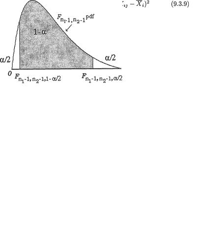
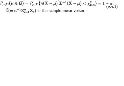
Example 9.4.1 Suppose that X1, ..., Xn are iid p–dimensional multivariate normal, Np(µ, Σ), random variables. Let us assume that the dispersion matrix Σ is p.d. and known. With given α (0, 1), we wish to derive a (1 – α) confidence region for the mean vector µ. Towards this end, from the Theorem 4.6.1, part (ii), let us recall that

Now, consider the non–negative expression 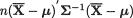as the pivot and denote

We write ,α for the upper 100α% point of the distribution, that is

=1-α. Thus, we define a p–dimensional confidence region Q for µ as follows:

One can immediately claim that

and hence, Q is a (1 – α) confidence region for the mean vector µ. Geometrically, the confidence region Q will be a p–dimensional ellipsoid having its center at the point , the sample mean vector. !

464 9. Confidence Interval Estimation

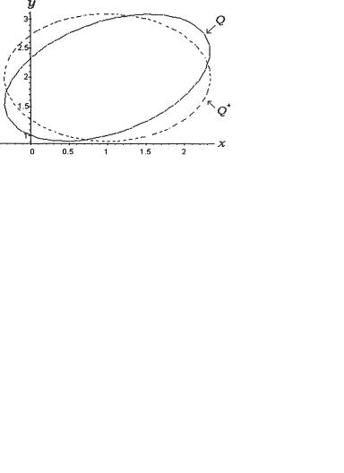
Figure 9.4.1. The Elliptic Confidence Regions Q from (9.4.3) and Q* from (9.4.4)

Example 9.4.2 (Example 9.4.1 Continued) Suppose that X1, ..., X10 are iid

fix α = .05, that is we require a 95% confidence region for µ. Now, one has

–2log(.05) = 5.9915. Suppose also that the observed value of ′ is (1, 2). Then, the confidence region from (9.4.2) simplifies to

which should be elliptic with its center at the point (1, 2). The Figure 9.4.1 gives a picture (solid curve) of the region Q which is the inner disk of the ellipse. The horizontal (x) and vertical (y) axis respectively correspond to µ1 and µ2.

fidence region for µ will also turn out to be elliptic with its center at the point (1, 2). Let us denote

The Figure 9.4.1 gives a picture (dotted curve) of the region Q* which is the inner disk of the ellipse. !

Example 9.4.3 Suppose that X1, ..., Xn are iid p–dimensional multivariate normal, Np(µ, Σ), random variables with n ≥ 2. Let us assume that the dispersion matrix Σ = σ2H where H is a p.d. and known matrix but the scale multiplier σ2( +), is unknown. With fixed α (0, 1), we wish to derive a (1 – α) confidence region for the mean vector µ.

Let us denote

which respectively estimate µ and σ2. Recall from Theorem 4.6.1, part (ii) that

One can show easily that

(pn – p)S2/s2 is distributed as and that the mean

Combining (9.4.5) and (9.4.6) we define the pivot

But, we note that we can rewrite U as

so that U has the Fp,pn–p distribution. We write Fp,pn–p,α for the upper 100α% point of the Fp,pn–p distribution, that is P{U < Fp,pn–p,α} = 1 – α. Thus, we define a p–dimensional confidence region Q for µ as follows:

Thus, we can immediately claim that

and hence Q is a (1 – α) confidence region for the mean vector µ. Again, geometrically the confidence region Q will be a p–dimensional ellipsoid with its center at the point . !

9.4.2Comparing the Means

Example 9.4.4 Suppose that Xi1, ..., Xin are iid random samples from the N(µi, σ2) population, i = 0, 1, ..., p. The observations X01, ..., X0n refer to a control with its mean µ0 whereas Xi1, ..., Xin are the observations from the ith treatment, i = 1, ..., p. Let us also assume that all the observations from the treatments and control are independent and that all the parameters are unknown.

466 9. Confidence Interval Estimation

The problem is one of comparing the treatment means µ1, ..., µp with the control mean µ0 by constructing a (1 – σ) joint confidence region for estimating the parametric function (µ1 – µ0, ..., µp – µ0). Let us denote

The random variables Y1, ..., Yn are obviously iid. Observe that any linear function of Yi is a linear function of the independent normal variables X1i, X2i,

..., Xpi and X0i. Thus, Y1, ..., Yn are iid p–dimensional normal variables. The common distribution is given by Np(µ, Σ) where

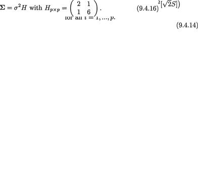
and Σ = σ2H where

Let us denote i = 0, 1, ..., p. The customary unbiased estimator of σ2 is the pooled sample variance,

and it is known that (p + 1)(n – 1)S2/σ2 is distributed as with the degree of freedom v = (p + 1)(n – 1). Also, S2 and are independently distributed, and hence S2 and are independently distributed. Next, let us consider the pivot

But, observe that is distributed as Np(0, Σ) where the correlation matrix

Thus, the pivot U has a multivariate t distribution, Mtp(v = (p &plus; 1)(n – 1), Σ), defined in Section 4.6.2. Naturally, we have the case of equicorrelation ρ where ρ = ½. So, we may determine a positive number h ≡ hv,α which is the upper equicoordinate 100α% point of the Mtp(v, Σ) distribution in the following sense:

The tables from Cornish (1954, 1962), Dunnett (1955), Dunnett and Sobel (1954, 1955), Krishnaiah and Armitage (1966), and Hochberg and Tamhane (1987) provide the values of “h” in various situations. For example, if α = .05 and p = 2, then from Table 5 of Hochberg and Tamhane (1987) we can read off h = 2.66, 2.54 respectively when n = 4, 5. Next, we simply rephrase (9.4.13) to make the following joint statements:

The simultaneous confidence intervals given by (9.4.14) jointly have 100(1 – α)% confidence. !

Example 9.4.5 Suppose that Xi1, ..., Xin are iid random samples from the N(µi, σ2) population, i = 1, ..., 4. The observations Xi1, ..., Xin, refer to the ith treatment, i = 1, ..., 4. Let us assume that all the observations from the treatments are independent and that all the parameters are unknown.

Consider, for example, the problem of jointly estimating the parameters θ1 = µ1 – µ2, θ2 = µ2 + µ3 – 2µ4 by means of a simultaneous confidence region. How should one proceed? Let us denote

The random variables Y1, ..., Yn are obviously iid. Also observe that any linear function of Yi is a linear function of the independent normal variables X1i, ..., X4i. Thus, Y1, ..., Yn are iid 2–dimensional normal variables. The common distribution is given by N2(θ, Σ) where θ ′ = (θ1, θ2) and

Now, along the lines of the Example 9.4.3, one can construct a 100(1 – α)% joint elliptic confidence region for the parameters θ1, θ2. On the other hand, one may proceed along the lines of the Example 9.4.4 to derive a 100(1 – α)% joint confidence intervals for the parameters θ1, θ2. The details are left out as Exercise 9.4.1. !

9.4.3Comparing the Variances

Example 9.4.6 Suppose that Xi1, ..., Xin are iid random samples from the population, i = 0, 1, ..., p. The observations X01, ..., X0n refer to a control population with its mean µ0 and variance σ20 whereas Xi1, ..., Xin

468 9. Confidence Interval Estimation

refer to the ith treatment, i = 1, ..., p. Let us also assume that the all observations from the treatments and control are independent.

The problem is one of comparing the treatment variances σ21,...,σ2p with the control variance σ20 by constructing a joint confidence region of the para-

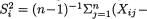
metric function Let us denote the ith sample variance which estimates i = 0, 1, ..., p. These sample variances are all independent and also is distributed as i =

0, 1, ..., p. Next, let us consider the pivot

which has a multivariate F distribution, M Fp(v0, v1, ..., vp) with v0 = v1 = ...

= vp = n – 1, defined in Section 4.6.3. With σ = (σ0, σ1, ..., σp), one may find a positive number b = bp,n,α such that

The Tables from Finney (1941) and Armitage and Krishnaiah (1964) will provide the b values for different choices of n and α. Next, we may rephrase (9.4.18) to make the following joint statements:

The simultaneous confidence intervals given by (9.4.19) jointly have 100(1 – α)% confidence. !

Example 9.4.7 (Example 9.4.6 Continued) From the pivot and its distribution described by (9.4.17), it should be clear how one may proceed to obtain the simultaneous (1 – α) two–sided confidence intervals for the variance ratios i = 1, ..., p. We need to find two positive numbers a and b , a < b, such that

so that with σ′ = (s0, s1, ..., sp) we have

Using (9.4.20), one can obviously determine simultaneous (1 – α) two–sided confidence intervals for all the variance ratios i = 1, ..., p. We leave the details out as Exercise 9.4.4.

4709. Confidence Interval Estimation

9.2.2Suppose that X has its pdf f(x; θ) = 2(θ – x)θ–2 I(0 < x < θ) where θ( +) is the unknown parameter. We are given α (0, 1). Consider the pivot U = X/θ and derive a (1 – α) two–sided confidence interval for θ.

9.2.3Suppose that X1, ..., Xn are iid Gamma(a, b) where a(> 0) is known but b(> 0) is assumed unknown. We are given α (0, 1). Find an appropriate pivot based on the minimal sufficient statistic and derive a two-sided (1 – α) confidence interval for b.

9.2.4Suppose that X1, ..., Xn are iid N(µ, σ2) where µ( ) is known but σ( +) is assumed unknown. We are given α (0, 1). We wish to obtain a (1 – α) confidence interval for σ.

(i) Find both upper and lower confidence intervals by inverting appropriate UMP level θ tests;

(ii) Find a two–sided confidence interval by considering an appropriate pivot based only on the minimal sufficient statistic.

9.2.5 Let X1, ..., Xn be iid with the common negative exponential pdf f(x; σ) = σ–1 exp{– (x – θ)/σ} I(x > θ). We suppose that θ( ) is known but σ( +) is unknown. We are given α (0, 1). We wish to obtain a (1 – θ) confidence interval for σ.

(i) Find both upper and lower confidence intervals by inverting appropriate UMP level θ tests;

(ii) Find a two–sided confidence interval by considering an appropriate pivot based only on the minimal sufficient statistic.

{Hint: The statistic is minimal sufficient for σ.}

9.2.6 Let X1, ..., Xn be iid with the common negative exponential pdf f(x; θ, σ) = σ–1 exp{– (x – θ)/σ} I(x > θ). We suppose that both the parameters θ( ) and σ( &plus;) are unknown. We are given α (0, 1). Find a (1 – θ) two-sided confidence interval for σ by considering an appropriate pivot based only on the minimal sufficient statistics. {Hint: Can a pivot be constructed

9.2.7Let X1, ..., Xn be iid with the common negative exponential pdf f(x; θ, σ) = σ–1 exp{ – (x – θ)/σ} I(x > θ). We suppose that both the parameters θ( ) and σ( &plus;) are unknown. We are given α (0, 1). Derive the joint (1 – α) two–sided confidence intervals for θ and σ based only on the minimal sufficient statistics. {Hint: Proceed along the lines of the Example 9.2.10.}

9.2.8Let X1, ..., Xn be iid Uniform(–θ, θ) where θ( +) is assumed unknown. We are given α (0, 1). Derive a (1 – α) two-sided confidence interval for θ based only on the minimal sufficient statistics. {Hint: Can

one justify working with |Xn:n| to come up with a suitable pivot?}

9.2.9 Let X1, ..., Xn be iid having the Rayleigh distribution with the common pdf f(x; θ) = 2θ–1 xexp(–x2/θ)I(x > 0) where θ(> 0) is the unknown parameter. We are given α (0, 1). First find both upper and lower (1 – α) confidence intervals for θ by inverting appropriate UMP level a tests. Next, consider an appropriate pivot and hence determine a (1 – α) two-sided confidence interval for θ based only on the minimal sufficient statistic.

9.2.10 Let X1, ..., Xn be iid having the Weibull distribution with the common pdf f(x; a) = a–1 bxb–1 exp(–xb/a)I(x > 0) where a(> 0) is an unknown parameter but b(> 0) is assumed known. We are given α (0, 1). First find both upper and lower (1 – α) confidence intervals for a by inverting appropriate UMP level α tests. Next, consider an appropriate pivot and hence determine a (1 – α) two–sided confidence interval for a based only on the minimal sufficient statistic.

9.2.12 (Exercise 9.2.7 Continued) Let X1, ..., Xn be iid with the common negative exponential pdf f(x; θ, σ) = σ–1 exp{–(x – θ)/σ}I(x > θ). We suppose that both the parameters θ( ) and σ( +) are unknown. We are given α (0, 1). In the Exercise 9.2.7, the joint (1 – α) two–sided confidence intervals for θ and σ were derived. From this, derive a confidence interval for each parametric function given below with the confidence coefficient at least (1 – α).

9.2.13A soda dispensing machine automatically fills the soda cans. The actual amount of fill must not vary too much from the target (12 fluid ounces) because the overfill will add extra cost to the manufacturer while the underfill will generate complaints from the customers. A random sample of 15 cans gave a standard deviation of .008 ounces. Assuming a normal distribution for the fill, estimate the true population variance with the help of a 95% two– sided confidence interval.

9.2.14Ten automobiles of the same make and model were tested by drivers with similar road habits, and the gas mileage for each was recorded over a week. The summary results were = 22 miles per gallon and s = 3.5 miles per gallon. Construct a 90% two–sided confidence interval for the true

472 9. Confidence Interval Estimation

average (µ) gas mileage per gallon. Assume a normal distribution for the gas mileage.

9.2.15 The waiting time (in minutes) at a bus stop is believed to have an exponential distribution with mean θ(> 0). The waiting times on ten occasions were recorded as follows:

(i) Construct a 95% two–sided confidence interval for the true average waiting time;

(ii) Construct a 95% two–sided confidence interval for the true variance of the waiting time;

(iii) At 5% level, is there sufficient evidence to justify the claim that the average waiting time exceeds 5 minutes?

9.2.16Consider a normal population with unknown mean µ and σ = 25.

How large a sample size n is needed to estimate µ within 5 units with 99% confidence?

9.2.17(Exercise 9.2.10 Continued) In the laboratory, an experiment was conducted to look into the average number of days a variety of weed takes to germinate. Twelve seeds of this variety of weed were planted on a dish. From the moment the seeds were planted, the time (days) to germination was recorded for each seed. The observed data follows:

The team’s expert in areas of soil and weed sciences believed that the time to germination had a Weibull distribution with its pdf

where a(> 0) is unknown but b = 3. Find a 90% two–sided confidence interval for the parameter a depending on the minimal sufficient statistic.

9.2.18 (Exercise 9.2.17 Continued) Before the lab experiment was conducted, the team’s expert in areas of soil and weed sciences believed that the average time to germination was 3.8 days. Use the confidence interval found in the Exercise 9.2.17 to test the expert’s belief. What are the respective null and alternative hypotheses? What is the level of the test?

9.3.1 (Example 9.3.1 Continued) Suppose that the random variables

Xi, ..., Xini are iid i = 1, 2, and that the X1j’s are independent of the X2j’s. Here we assume that the means µ1, µ2 are unknown but σ1, σ2

are known, (µi, σi) × +, i = 1, 2. With fixed α (0, 1), construct a

(1 – α) two–sided confidence interval for µ1 – µ2 based on sufficient statistics for (µ1, µ2). Is the interval shortest among all (1 – α) two–sided confidence intervals for µ1 – µ2 depending only on the sufficient statistics for

(µ1, µ2)?

9.3.2 (Example 9.3.1 Continued) Suppose that the random variables Xi1,

..., Xini are iid N(µi, kiσ2), ni ≥ 2, i = 1, 2, and that the X1j’s are independent of the X2j’s. Here we assume that all three parameters µ1, µ2, σ are unknown

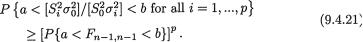
but k1, k2 are positive and known, (µ1, µ2, σ) × × +. With fixed α (0, 1), construct a (1 – α) two–sided confidence interval for µ1 – µ2 based on sufficient statistics for (µ1, µ2, σ). Is the interval shortest on the average among all (1 – α) two–sided confidence intervals for µ1 – µ2 depending on sufficient statistics for (µ , µ , σ)? {Hint: Show that the sufficient statistic is

σ). {Hint: Combine the separate estimation problems for (µ1 – µ2) and σ via the Bonferroni inequality.}

9.3.6 Two types of cars were compared for their braking distances. Test runs were made for each car in a driving range. Once a car reached the stable speed of 60 miles per hour, the brakes were applied. The distance

474 9. Confidence Interval Estimation

(feet) each car travelled from the moment the brakes were applied to the moment the car came to a complete stop was recorded. The summary statistics are shown below:

Construct a 95% two–sided confidence interval for µB – µA based on sufficient statistics. Assume that the elapsed times are distributed as N(µA, σ2) and N(µB, σ2) respectively for the Make A and B cars with all parameters unknown. Is the interval shortest on the average among all 95% two–sided confidence intervals for µB – µA depending on sufficient statistics for (µA, µB, σ)?

9.3.7 In an experiment in nutritional sciences, a principal investigator considered 8 overweight men with comparable backgrounds which included eating habits, family traits, health condition and job related stress. A study was conducted to estimate the average weight reduction for overweight men following a regimen involving nutritional diet and exercise. The technician weighed in each individual before they entered this program. At the conclusion of the two–month long study, each individual was weighed. The data follows:

Here, it is not reasonable to assume that in the relevant target population, X1 and X2 are independent. The nutritional scientist believed that the assumption of a bivariate normal distribution would be more realistic. Obtain a 95% two– sided confidence interval for µ1 – µ2 where E(Xi) = µi, i = 1, 2.

9.3.8 (Exercise 9.3.7 Continued) Suppose that the scientist believed before running this experiment that on the average the weight would go down by at least 10 pounds when such overweight men went through their regimen of diet and exercise for a period of two months. Can the 95% confidence

interval found in the Exercise 9.3.7 be used to test the scientist’s belief at 5% level? If not, then find an appropriate 95% confidence interval for µ1 – µ2 in the Exercise 9.3.7 and use that to test the hypothesis at 5% level.

9.3.9 Two neighboring towns wanted to compare the variations in the time (minutes) to finish a 5k–run among the first place winners during each town’s festivities such as the heritage day, peach festival, memorial day, and other town–wide events. The following data was collected recently by the town officials:

Assume that the performances of these first place winners are independent and that the first place winning times are normally distributed within each town’s festivities. Obtain a 90% two–sided confidence interval for σA/σB based on sufficient statistics for (µA, µB, σA, σB). Can we conclude at 10%

level that σA = σB?

9.3.10 Suppose that the random variables Xi1, ..., Xini are iid having the common pdf f(x; θi), i = 1, 2, where we denote the exponential pdf f(x; a) = a–1 exp{–x/a}I(x > 0), a +. Also, let the X1j’s be independent of the X2j’s. We assume that both the parameters θ1, θ2 are unknown, (θ1, θ2) + × +. With fixed α (0, 1), derive a (1 – α) two-sided confidence interval for θ2/θ1 based on sufficient statistics for (θ1, θ2). {Hint: Consider creating a pivot out

of

9.3.11 (Example 9.3.6 Continued) Suppose that the random variables Xi1,

..., Xin are iid Uniform(0, θi), i = 1, 2. Also, let the X1j’s be independent of the X2j’s. We assume that both the parameters are unknown, (θ1, θ2) + × +. With fixed α (0, 1), derive a (1 – α) two-sided confidence interval for θ1/ (θ1 + θ2) based on sufficient statistics for (θ1, θ2).

9.4.1 (Example 9.4.5 Continued) Suppose that Xi1, ..., Xin are iid random samples from the N(µi, σ2) population, i = 1, ..., 4. The observations Xi1, ..., Xin refer to the ith treatment, i = 1, ..., 4. Let us assume that the treatments are independent too and that all the parameters are unknown. With fixed α (0, 1), derive the (1 – α) joint confidence intervals for estimating the parameters

θ1 = µ1 – µ2, θ2 = µ2 + µ3 – 2µ4.

9.4.2 (Example 9.4.4 Continued) Suppose that Xi1, ..., Xin are iid random samples from the N(µi, σ2) population, i = 1, ..., 5. The observations Xi1, ..., Xin refer to the ith treatment, i = 1, ..., 5. Let us assume that the treatments are independent too and that all the parameters are unknown. With fixed α (0, 1), derive the (1 – α) joint ellipsoidal confidence region for estimating the parameters θ1 = µ1 – µ2, θ2 = µ2 – µ3 and θ3 = µ3 + µ4 – 2µ5.

4769. Confidence Interval Estimation

9.4.3(Exercise 9.4.2 Continued) Suppose that Xi1, ..., Xin are iid random samples from the N(µi, σ2) population, i = 1, ..., 5. The observations Xi1, ..., Xin refer to the ith treatment, i = 1, ..., 5. Let us assume that the treatments are independent too and that all the parameters are unknown. With fixed α (0, 1), derive the (1 – α) joint confidence intervals for estimating the parameters

θ1 = µ1 – µ2, θ2 = µ2 – µ3 and θ3 = µ3 + µ4 – 2µ5.

9.4.4 Use the equation (9.4.20) to propose the simultaneous (1 – α) twosided confidence intervals for the variance ratios.

9.4.5 Let Xi1, ..., Xin be iid having the common pdf f(x; µi, σi), n ≥ 2, where f(x; µ, σ) = σ–1 exp{–(x – µ)/σ}I(x > µ), (µi, σi) × +, i = 0, 1,

..., p. The observations X01, ..., X0n refer to a control whereas Xi1, ..., Xin refer to the ith treatment, i = 1, ..., p. Suppose that all the observations are independent and all the parameters are unknown. Start with an appropriate p– dimensional pivot depending on the sufficient statistics and then, with fixed α(0, 1), derive the simultaneous (1 – α) two-sided confidence intervals for the ratios σi/σ0, i = 1, ..., p. {Hint: Proceed along the lines of the Examples 9.4.6–9.4.7.}

9.4.6 (Exercise 9.3.10 Continued) Suppose that the random variables Xi1,

..., Xin are iid having the common pdf f(x; θi) where we denote the exponential pdf f(x; a) = a–1 exp{–x/a}I(x > 0), θi > 0, i = 0, 1, ..., p. The observations X01, ..., X0n refer to a control whereas Xi1, ..., Xin refer to the ith treatment, i = 1, ..., p. Suppose that all the observations are independent and all the parameters are unknown. Start with an appropriate p–dimensional pivot depending on the sufficient statistics and then, with fixed α (0, 1), derive the simultaneous (1 – α) two-sided confidence intervals for the ratios θi/θ0, i = 1, ..., p. {Hint: Proceed along the lines of the Examples 9.4.6–9.4.7.}