

3
Multivariate Random Variables
3.1 Introduction
Suppose that we draw two random digits, each from the set {0, 1, ..., 9}, with equal probability. Let X1, X2 be respectively the sum and the difference of the two selected random digits. Using the sample space technique, one can easily verify that P(X1 = 0) = 1/100, P(X1 = 1) = 2/100, P(X1 = 2) = 3/100 and eventually obtain the distribution, namely P(X1 = i) for i = 0, 1,
..., 18. Similarly, one can also evaluate P(X2 = j) for j = –9, –8, ..., 8, 9. Now, suppose that one has observed X1 = 3. Then there is no chance for X2 to take a value such as 2. In other words, the bivariate discrete random variable (X1, X2) varies together in a certain way. This sense of joint variation is the subject matter of the present chapter.
Generally speaking, we may have k(≥ 2) real valued random variables X1,
..., Xk which vary individually as well as jointly. For example, during the “health awareness week” we may consider a population of college students and record a randomly selected student’s height (X1), weight (X2), age (X3) and blood pressure (X4). Each individual random variable may be assumed to follow some appropriate probability distribution in the population, but it may also be quite reasonable to assume that these four variables together follow a certain joint probability distribution. This example falls in the category of multivariate continuous random variables.
The Section 3.2 introduces the ideas of joint, marginal and conditional distributions in a discrete situation including the multinomial distribution. The Section 3.3 introduces analogous topics in the continuous case. We begin with the bivariate scenario for simplicity. The notion of a compound distribution and the evaluation of the associated mean and variance are explored in the Examples 3.3.6-3.3.8. Multidimensional analysis is included in the Section 3.3.2. The notions of the covariances and correlation coefficients between random variables are explored in the Section 3.4. We briefly revisit the multinomial distribution in the Section 3.4.1. The Section 3.5 introduces the concept of the independence of random variables. The celebrated bivariate normal distribution is discussed in the Section 3.6 and the associated marginal as well as the conditional pdf’s are found in this special situation. The relationships between the zero correlation and possible
99
100 3. Multivariate Random Variables
independence are explained in the Section 3.7. The Section 3.8 summarizes both the one- and multi-parameter exponential families of distributions. This chapter draws to an end with some of the standard inequalities which are widely used in statistics. The Sections 3.9.1-3.9.4 include more details than Sections 3.9.5-3.9.7.
3.2 Discrete Distributions
Let us start with an example of bivariate discrete random variables.
Example 3.2.1 We toss a fair coin twice and define Ui = 1 or 0 if the ith toss results in a head (H) or tail (T), i = 1, 2. We denote X1 = U1 + U2 and X2 = U1
– U2. Utilizing the techniques from the previous chapters one can verify that X1 takes the values 0, 1 and 2 with the respective probabilities 1/4, 1/2 and 1/ 4, whereas X2 takes the values –1, 0 and 1 with the respective probabilities 1/ 4, 1/2 and 1/4. When we think of the distribution of Xi alone, we do not worry much regarding the distribution of Xj, i ≠ j = 1, 2. But how about studying the random variables (X1, X2) together? Naturally, the pair (X1, X2) takes one of the nine (= 32) possible pairs of values: (0, –1), (0, 0), (0, 1), (1, –1), (1, 0), (1, 1), (2, –1), (2, 0), and (2, 1).
Table 3.2.1. Joint Distribution of X1 and X2
|
|
X1 values |
|
Row Total |
|
0 |
1 |
2 |
|
–1 |
|
|
|
.25 |
0 |
.25 |
0 |
||
X2 values 0 |
.25 |
0 |
.25 |
.50 |
1 |
0 |
.25 |
0 |
.25 |
Col. Total |
|
|
|
|
.25 |
.50 |
.25 |
1.00 |
|
|
|
|
|
|
Note that X1 = 0 implies that we must have observed TT, in other words U1 =
U2 = 0, so that P(X1 = 0 ∩ X2 = 0) = P(TT) = 1/4. Whereas P(X1 = 0 ∩ X2 = –1) = P(X1 = 0 ∩ X2 = 1) = 0. Other entries in the Table 3.2.1 can be verified
in the same way. The entries in the Table 3.2.1 provide the joint probabilities, P(X1 = i ∩ X2 = j) for all i = 0, 1, 2 and j = –1, 0, 1. Such a representation is provides what is known as the joint distribution of X1, X2. The column and row totals respectively line up exactly with the individual distributions of X1, X2 respectively which are also called the marginal distributions of X1, X2.!

3. Multivariate Random Variables |
101 |
3.2.1 TheJoint,MarginalandConditionalDistributions
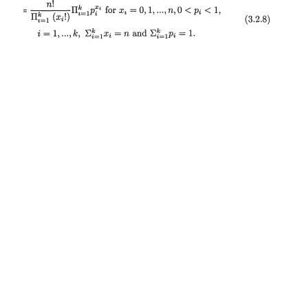
Suppose that we have k(≥ 2) discrete random variables X1, ..., Xk where Xi takes one of the possible values xi belonging to its support χi, i = 1, ..., k. Here, χi can be at most countably infinite. The joint probability mass function (pmf) of X = (X1, ..., Xk) is then given by
A function such as f(x) would be a genuine joint pmf if and only if the following two conditions are met:
These are direct multivariable extensions of the requirements laid out earlier in (1.5.3) in the case of a single real valued random variable.
The marginal distribution of Xi corresponds to the marginal probability mass function defined by
Example 3.2.2 (Example 3.2.1 Continued) We have χ1 = {0, 1, 2}, χ2 = {–1, 0, 1}, and the joint pmf may be summarized as follows: f(x1, x2) = 0 when (x1, x2) = (0, –1), (0, 1), (1, 0), (2, –1), (2, 1), but f(x1, x2) = .25 when (x1, x2) = (0, 0), (1, –1), (1, 1), (2, 0). Let us apply (3.2.3) to obtain the marginal pmf of X1.
which match with the respective column totals in the Table 3.2.1. Similarly, the row totals in the Table 3.2.1 will respectively line up exactly with the marginal distribution of X2. !
In the case of k-dimensions, the notation becomes cumbersome in defining the notion of the conditional probability mass functions. For simplicity, we explain the idea only in the bivariate case.
102 3. Multivariate Random Variables
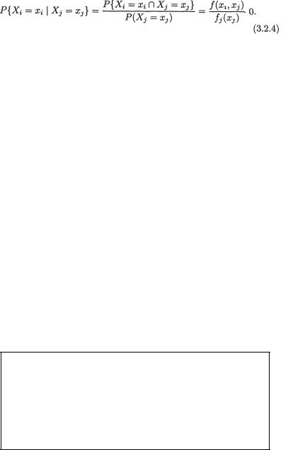
For i≠ j, the conditional pmf of Xi at the point xi given that Xj = xj, denoted by fi|j(xi), is defined by
Now, suppose that P(Xj = xj), which is equivalent to fj(xj), is positive. Then, using the notion of the conditional probability from (1.4.1) we can express
fi|j(xi) as
for xi χi, i ≠ j. In the two-dimensional case, we have two conditional pmf’s, namely f1|2(x1) and f2|1(x2) which respectively represent the conditional pmf of X1 given X2 = x2 and that of X2 given X1 = x1.
Once the conditional pmf f1|2(x1) of X1 given X2 = x2 and the conditional pmf f2|1(x2) of X2 given X1 = x1 are found, the conditional mean of Xi given Xj = xj, denoted by E[Xi | Xj = xj], is defined as follows:
This is not really any different from how we interpreted the expected value of a random variable in the Definition 2.2.1. To find the conditional expectation of Xi given Xj = xj, we simply multiply each value xi by the conditional probability P{Xi = xi | Xj = xj} and then sum over all possible values xi χi with any fixed xj χj, for i ≠ j = 1, 2.
Example 3.2.3 (Example 3.2.2 Continued) One can verify that given X2 = –1, the conditional pmf f1|2(x1) corresponds to 0, 1 and 0 respectively when x1 = 0, 1, 2. Other conditional pmf’s can be found analogously. !
Example 3.2.4 Consider two random variables X1 and X2 whose joint distribution is given as follows:
Table 3.2.2. Joint Distribution of X1 and X2
|
|
X1 values |
|
Row Total |
|
–1 |
2 |
|
5 |
1 |
|
|
|
.55 |
.12 |
.18 |
.25 |
||
X2 values |
|
|
|
|
2 |
.20 |
.09 . |
16 |
.45 |
Col. Total |
|
|
|
1.00 |
.32 |
.27 |
.41 |
3. Multivariate Random Variables |
103 |
One has χ1 = {–1, 2, 5}, χ2 = {1, 2}. The marginal pmf’s of X1, X2 are respectively given by f1(–1) = .32, f1(2) = .27, f1(5) = .41, and f2(1) = .55, f2(2) = .45. The conditional pmf of X1 given that X2 = 1, for example, is given
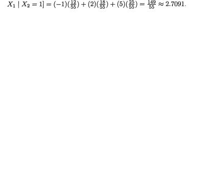
by f1|2(–1) = 12/55, f1|2(2) = 18/55, f1|2(5) = 25/55. We can apply the notion of the conditional expectation from (3.2.5) to evaluate E[X1 | X2 = 1] and write
That is, the conditional average of X1 given that X2 = 1 turns out to be approximately 2.7091. Earlier we had found the marginal pmf of X1 and hence we have
Obviously, there is a conceptual difference between the two expressions E[X1] and E[X1 | X2 = 1]. !
If we have a function g(x1, x2) of two variables x1, x2 and we wish to evaluate E[g(X1, X2)], then how should we proceed? The approach involves a simple generalization of the Definition 2.2.3. One writes
Example 3.2.5 (Example 3.2.4 Continued) Suppose that g(x1, x2) = x1x2 and let us evaluate E[g(X1, X2)]. We then obtain
Instead, if we had , then one can similarly check that E[h(X1, X2)] = 16.21. !
3.2.2The Multinomial Distribution
Now, we discuss a special multivariate discrete distribution which appears in the statistical literature frequently and it is called the multinomial distribution. It is a direct generalization of the binomial setup introduced earlier in (1.7.2). First, let us look at the following example.
Example 3.2.6 Suppose that we have a fair die and we roll it twenty times. Let us define Xi = the number of times the die lands up with the face having i dots on it, i = 1, ..., 6. It is not hard to see that individually
104 3. Multivariate Random Variables
Xi has the Binomial (20, 1/6) distribution, for every fixed i = 1, ..., 6. It is clear, however, that  must be exactly twenty in this example and hence we conclude that X1, ..., X6 are not all free-standing random variables. Suppose that one has observed X1 = 2, X2 = 4, X3 = 4, X5 = 2 and X6 = 3, then X4 must be 5. But, when we think of X4 alone, its marginal distribution is Binomial (20, 1/6) and so by itself it can take any one of the possible values 0, 1, 2, ..., 20. On the other hand, if we assume that X1 = 2, X2 = 4, X3 = 4, X5 = 2 and X6 = 3, then X4 has to be 5. That is to say that there is certainly some kind of dependence among these random variables X1, ..., X6. What is the exact nature of this joint distribution? We discuss it next. !
We denote a vector valued random variable by X = (X1, ..., Xk) in general. A discrete random variable X is said to have a multinomial distribution involving n and p1, ..., pk, denoted by Multk(n, p1, ..., pk), if and only if the joint pmf of X is given by
We may think of the following experiment which gives rise to the multinomial pmf. Let us visualize k boxes lined up next to each other. Suppose that we have n marbles which are tossed into these boxes in such a way that each marble will land in one and only one of these boxes. Now, let pi stand for the probability of a marble landing in the ith box, with 0 < pi < 1, i = 1, ..., k,  . These p’s are assumed to remain same for each tossed marble. Now, once these n marbles are tossed into these boxes, let Xi = the number of marbles which land inside the box ≠i, i = 1, ..., k. The joint distribution of X = (X1, ..., Xk) is then characterized by the pmf described in (3.2.8).
How can we verify that the expression given by (3.2.8) indeed corresponds to a genuine pmf? We must check the requirements stated in (3.2.2). The first requirement certainly holds. In order to verify the requirement (ii), we need an extension of the Binomial Theorem. For completeness, we state and prove the following result.
Theorem 3.2.1 (Multinomial Theorem) Let a1, ..., ak be arbitrary real numbers and n be a positive integer. Then, we have
3. Multivariate Random Variables |
105 |
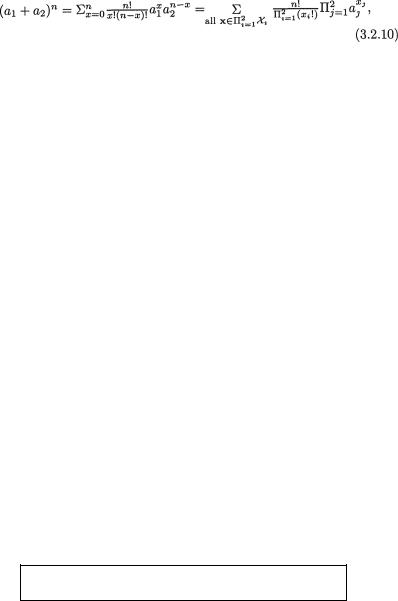
Proof First consider the case k = 2. By the Binomial Theorem, we get
which is the same as (3.2.9). Now, in the case k = 3, by using (3.2.10) repeatedly let us write
which is the same as (3.2.9). Next, let us assume that the expansion (3.2.9) holds for all n ≤r, and let us prove that the same expansion will then hold for n = r + 1. By mathematical induction, the proof will then be complete. Let us write
which is the same as (3.2.9). The proof is now complete. ¢
The fact that the expression in (3.2.8) satisfies the requirement (ii) stated in (3.2.2) follows immediately from the Multinomial Theorem. That is, the function f(x) given by (3.2.8) is a genuine multivariate pmf.
The marginal distribution of the random variable Xi is
Binomial (n,pi) for each fixed i = 1, ..., k.
In the case of the multinomial distribution (3.2.8), suppose that we focus on the random variable Xi alone for some arbitrary but otherwise fixed
106 3. Multivariate Random Variables
i = 1, ..., k. The question is this: Out of the n marbles, how many (that is, Xi) would land in the ith box? We are simply counting how many marbles would fall in the ith box and how many would fall outside, that is in any one of the other k
– 1 boxes. This is the typical binomial situation and hence we observe that the random variable Xi has the Binomial(n, pi) distribution for each fixed i = 1, ..., k. Hence, from our discussions on the binomial distribution in Section 2.2.2 and (2.2.17), it immediately follows that
Example 3.2.7 (Example 3.2.6 Continued) In the die rolling example, X = (X1, ..., Xk) has the Multk(n, p1, ..., pk) distribution where n = 20, k = 6, and p1 = ... = p6 = 1/6. !
The derivation of the moment generating function (mgf) of the multinomial distribution and some of its applications are highlighted in Exercise 3.2.8.
The following theorems are fairly straightforward to prove. We leave their proofs as the Exercises 3.2.5-3.2.6.
Theorem 3.2.2 Suppose that the random vector X = (X1, ..., Xk) has the Multk(n, p1, ..., pk) distribution. Then, any subset of the X variables of size
r, namely (Xi1, ..., Xir) has a multinomial distribution in the sense that (Xi1, ...,
Xir, |
) is Multr+1(n, pi1, ..., pir, |
) where 1 ≤ i1 < i2 < ... < ir ≤ k |
and |
|
|
Theorem 3.2.3 Suppose that the random vector X = (X1, ..., Xk) has the Multk(n, p1, ..., pk) distribution. Consider any subset of the X variables of size r, namely (Xi1, ..., Xir). The conditional joint distribution of (Xi1, ..., Xir) given all the remaining X’s is also multinomial with its conditional pmf
Example 3.2.8 (Example 3.2.7 Continued) In the die rolling example, suppose that we are simply interested in counting how many times the faces with the numbers 1 and 5 land up. In other words, our focus is on the three

3. Multivariate Random Variables |
107 |
dimensional random variable (X1, X5,  ) where
  ).By the Theorem 3.2.2, the three dimensional variable of interest (X1, X5,
 )has the Mult3(n, 1/6, 1/6, 2/3) distribution where n = 20. !
3.3 Continuous Distributions
Generally speaking, we may be dealing with k(≥ 2) real valued random variables X1, ..., Xk which vary individually as well as jointly. We may go back to the example cited earlier in the introduction. Consider a population of college students and record a randomly selected student’s height (X1), weight (X2), age (X3), and blood pressure (X4). It may be quite reasonable to assume that these four variables together has some multivariate continuous joint probability distribution in the population.
The notions of the joint, marginal, and conditional distributions in the case of multivariate continuous random variables are described in the Section 3.3.1. This section begins with the bivariate scenario for simplicity. The notion of a compound distribution and the evaluation of the associated mean and variance are explored in the Examples 3.3.6-3.3.8. Multidimensional analysis is included in the Section 3.3.2.
3.3.1The Joint, Marginal and Conditional Distributions
For the sake of simplicity, we begin with the bivariate continuous random variables. Let X1, X2 be continuous random variables taking values respectively in the spaces χ1, χ2 both being subintervals of the real line . Consider a function f(x1, x2) defined for (x1, x2) χ1 × χ2. Throughout we will use the following convention:
Let us presume that χ1 × χ2 is the support of the probability
distribution in the sense that f(x1, x2) > 0 for all (x1, x2)χ1 × χ2 and f(x1, x2) = for all (x1, x2) 2 – (χ1 × χ2).
Such a function f(x1, x2) would be called a joint pdf of the random vector X = (X1, X2) if the following condition is satisfied:
Comparing (3.3.1) with the requirement (ii) in (3.2.2) and (1.6.1), one will notice obvious similarities. In the case of one-dimensional random variables, the integral in (1.6.1) was interpreted as the total area under the density curve y = f(x). In the present situation involving two random
108 3. Multivariate Random Variables
variables, the integral in (3.3.1) will instead represent the total volume under the density surface z = f(x1, x2).
The marginal distribution of one of the random variables is obtained by integrating the joint pdf with respect to the remaining variable. The marginal pdf of Xi is then formally given by
Visualizing the notion of the conditional distribution in a continuous scenario is little tricky. In the discrete case, recall that fi(xi) was simply interpreted as P(Xi = xi) and hence the conditional pmf was equivalent to the corresponding conditional probability given by (3.2.4) as long as P(Xi = x1) > 0. In the continuous case, however, P(Xi = xi) = 0 for all xi χi with i = 1, 2. So, conceptually how should one proceed to define a conditional pdf?
Let us first derive the conditional df of X1 given that x2≤ X2 ≤ x2 + h where h(> 0) is a small number. Assuming that P(x2 ≤X2 ≤x2 + h) > 0, we have
From the last step in (3.3.3) it is clear that as h ↓ 0, the limiting value of this conditional probability takes the form of 0/0. Thus, by appealing to the L’Hôpital’s rule from (1.6.29) we can conclude that
Next, by differentiating the last expression in (3.3.4) with respect to x1, one obtains the expression for the conditional pdf of X1 given that X2 = x2.
3. Multivariate Random Variables |
109 |
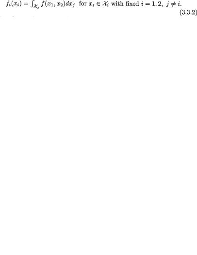
Hence, the conditional pdf of X1 given that X2 = x2 is given by
Once these conditional pdf’s are obtained, one can legitimately start talking about the conditional moments of one of the random variables given the other. For example, in order to find the conditional mean and the conditional variance of X1 given that X2 = x2, one should proceed as follows:
It should be clear that µ1/2 and  respectively from (3.3.7) would corre-
spond to the conditional mean and the conditional variance of X1 given that
X2 = x2. In general, we can write
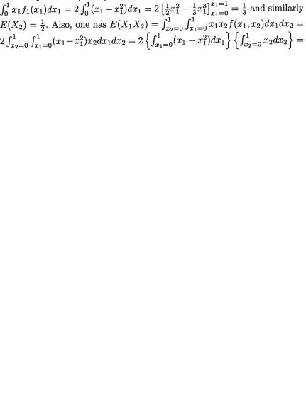
Example 3.3.1 Consider two random variables X1 and X2 whose joint continuous distribution is given by the following pdf:
Obviously, one has χ1 = χ2 = (0, 1). Next, we integrate this joint pdf with respect to x2 to obtain the marginal pdf of X1 and write
for 0 < x1 < 1. In the same fashion, we obtain the marginal pdf of X2 as follows:
110 3. Multivariate Random Variables
for 0 < x2 < 1. Next, we can simply use the marginal pdf f2(x2) of X2 to obtain
so that
The reader may similarly evaluate E(X1) and V(X1). !
Example 3.3.2 (Example 3.3.1 Continued) One should easily verify that
are respectively the two conditional pdf’s. For fixed 0 < x1 < 1, the conditional expectation of X2 given that X1 = x1 is obtained as follows:
One can evaluate the expression  of as follows:
so that using (3.3.14) and after considerable simplifications, we find:
The details are left out as Exercise 3.3.1.!
Example 3.3.3 Consider two random variables X1 and X2 whose joint continuous distribution is given by the following pdf:
Obviously, one has χ1 = χ2 = (0, 1). One may check the following expressions for the marginal pdf’s easily:
3. Multivariate Random Variables |
111 |
One should derive the conditional pdf’s and the associated conditional means and variances. See the Exercise 3.3.2. !
In a continuous bivariate distribution, the joint, marginal, and conditional pdf’s were defined in (3.3.1)-(3.3.2) and (3.3.5)-(3.3.6).
In the case of a two-dimensional random variable, anytime we wish to calculate the probability of an event A( 2), we may use an approach which is a generalization of the equation (1.6.2) in the univariate case: One would write
We emphasize that the convention is to integrate f(x1, x2) only on that part of the set A where f(x1, x2) is positive.
If we wish to evaluate the conditional probability of an event B( ) given, say, X1 = x1, then we should integrate the conditional pdf f2/1(x2) of X2
given X1 = x1 over that part of the set B where f2/1(x2) is positive. That is, one has
Example 3.3.4 (Example 3.3.2 Continued) In order to appreciate the essence of what (3.3.20) says, let us go back for a moment to the Example 3.3.2. Suppose that we wish to find the probability of the set or
the event A where A = {X1 = .2 ∩.3 < X2 = .8}. Then, in view of (3.3.20), we obtain
dx1 = 1.2(.845 – .62) = .27. !
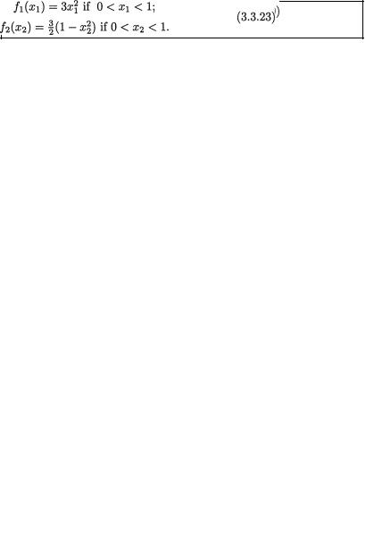
Example 3.3.5 Consider two random variables X1 and X2 whose joint continuous distribution is given by the following pdf:
Obviously, one has χ1 = χ2 = (0, 1). One may easily check the following expressions for the marginal pdf’s:
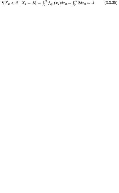
Now, suppose that we wish to compute the conditional probability that X2 < .2 given that X1 = .5. We may proceed as follows. We have
112 3. Multivariate Random Variables
and hence using (3.3.24), one can write
One may, for example, evaluate µ2/1 too given that X1 = .5. We leave it out as the Exercise 3.3.3. !
We defined the conditional mean and variance of a random variable X1 given the other random variable X2 in (3.3.7). The following result gives the tool for finding the unconditional mean and variance of X1 utilizing the expressions of the conditional mean and variance.
Theorem 3.3.1 Suppose that X = (X1, X2) has a bivariate pmf or pdf, namely f(x1, x2) for xi χi, the support of Xi, i = 1, 2. Let E1[.] and V1[.] respectively denote the expectation and variance with respect to the marginal distribution of X1. Then, we have
(i)E[X2] = E1[E2/1 {X2 | X1}];
(ii)V(X2) = V1[E2/1{X2 | X1}] + E1[V1/V2/1{X2 | X1}].
Proof (i) Note that
Next, we can rewrite
which is the desired result.
(ii) In view of part (i), we can obviously write
where g(x1) = E{(X2 – χ2)2 | X1 = x1}. As before, denoting E{X2 | X1 = x1} by µ2/1, let us rewrite the function g(x1) as follows:

3. Multivariate Random Variables |
113 |
But, observe that the third term in the last step (3.3.29) can be simplified as follows:
which is zero. Now, we combine (3.3.29)-(3.3.30) and obtain
At this point, (3.3.31) combined with (3.3.29) then leads to the desired result stated in part (ii). ¢
The next three Examples 3.3.6-3.3.8, while applying the Theorem 3.3.1, introduce what are otherwise known in statistics as the compound distributions.
Example 3.3.6 Suppose that conditionally given X1 = x1, the random variable X2 is distributed as N(β0 + β1x1,  ) for any fixed x1 . Here, β0, β1 are
two fixed real numbers. Suppose also that marginally, X1 is distributed as N(3, 10). How should we proceed to find E[X2] and V[X2]? The Theorem 3.3.1 (i) will immediately imply that
which reduces to β0 + 3β1. Similarly, the Theorem 3.3.1 (ii) will imply that
which reduces to Refer to the Section 2.3.3 as needed. In a situation like this, the marginal distribution of X2 is referred to as a compound distribution. Note that we have been able to derive the expressions of the mean and variance of X2 without first identifying the marginal distribution of
X2. !
Example 3.3.7 Suppose that conditionally given X1 = x1, the random variable X2 is distributed as Poisson (x1) for any fixed x1 +. Suppose also that marginally, X1 is distributed as Gamma (α = 3, β = 10). How should we proceed to find E[X2] and V[X2]? The Theorem 3.3.1 (i) will immediately imply that

114 3. Multivariate Random Variables
Similarly, the Theorem 3.3.1 (ii) will imply that
which reduces to 330. Refer to the Sections 2.3.2 and 2.3.4 as needed. In a situation like this, again the marginal distribution of X2 is referred to as a compound distribution. Note that we have been able to derive the expressions of the mean and variance of X2 without first identifying the marginal distribution of X2. !
Example 3.3.8 Suppose that conditionally given X1 = x1, the random variable X2 is distributed as Binomial(n, x1) for any fixed x1 (0, 1). Suppose also that marginally, X1 is distributed as Beta(α = 4, β = 6). How should we proceed to find E[X2] and V[X2]? The Theorem 3.3.1 (i) will immediately imply that
Similarly, the Theorem 3.3.1 (ii) will imply that
Refer to the Sections 2.3.1 and equation (1.7.35) as needed. One can verify
that |
Also, we have . |
Hence,
we have
In a situation like this, again the marginal distribution of X2 is referred to as a compound distribution. Note that we have been able to derive the expressions of the mean and variance of X2 without first identifying the marginal distribution of X2. !
Example 3.3.9 (Example 3.3.2 Continued) Let us now apply the Theorem 3.3.1 to reevaluate the expressions for E[X2] and V[X2]. Combining (3.3.15) with the Theorem 3.3.1 (i) and using direct integration with respect

3. Multivariate Random Variables |
115 |
to the marginal pdf f1(x1) of X1 from (3.3.10), we get
which matches with the answer found earlier in (3.3.12). Next, combining (3.3.15) and (3.3.17) with the Theorem 3.3.1 (ii), we should then have
Now, we combine (3.3.39) and (3.3.40). We also use the marginal pdf f1(x1) of X1 from (3.3.10) and direct integration to write
since E[(1 – X1)] = 3/4 and E[(1 – X1)2] = 3/5. The answer given earlier in (3.3.13) and the one found in (3.3.41) match exactly. !
3.3.2 Three and Higher Dimensions
The ideas expressed in (3.3.2) and (3.3.5)-(3.3.6) extend easily in a multivariate situation too. For example, let us suppose that a random vector X =
(X1, X2, X3, X4) has the joint pdf f(x1, x2, x3, x4) where xi χi, the support of Xi, i = 1, 2, 3, 4. The marginal pdf of (X1, X3), that is the joint pdf of X1 and
X3, for example, can be found as follows:
The conditional pdf of (X2, X4) given that X1 = x1, X3 = x3 will be of the form
and the x’s belong to the χ’s. The notions of expectations and conditional expectations can also be generalized in a natural fashion in the case of a
116 3. Multivariate Random Variables
multidimensional random vector X by extending the essential ideas from (3.3.7)- (3.3.8).
If one has a k-dimensional random variable X = (X1, ..., Xk), the joint pdf would then be written as f(x) or f(x1, ..., xk). The joint pdf of any subset of random variables, for example, X1 and X3, would then be found by integrating f(x1, ..., xk) with respect to the remaining variables x2, x4, ..., xk. One can also write down the expressions of the associated conditional pdf’s of any subset of random variables from X given the values of any other subset of random variables from X.
Theorem 3.3.2 Let X = (X1, ..., Xk) be any k-dimensional discrete or continuous random variable. Suppose that we also have real valued functions hi(x) and constants ai, i = 0, 1, ..., p. Then, we have
as long as all the expectations involved are finite. That is, the expectation is a linear operation.
Proof Let us write  and hence we have
Now, the proof is complete. ¢
Next, we provide two specific examples.
Example 3.3.10 Let us denote χ1 = χ3 = (0, 1), χ2 = (0, 2) and define
Note that these are non-negative functions and ∫χi ai(xi)dxi = 1 for all
3. Multivariate Random Variables |
117 |
i = 1, 2, 3. With x = (x1, x2, x3)  and , let us denote
Now, one can easily see that
and
Hence, for the function f(x) defined in (3.3.47) we have
and also observe that f(x) is always non-negative. In other words, f(x) is a pdf of a three dimensional random variable, say, X = (X1, X2, X3). The joint pdf of X1, X3 is then given by
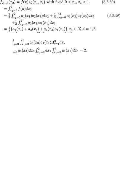
One may directly check by double integration that g(x1, x3) is a genuine pdf with its support being χ1 × χ3. For any 0 < x2 < 2, with g(x1, x3) from (3.3.49), the conditional pdf of X2 given that X1 = x1, X3 = x3 is then given by

118 3. Multivariate Random Variables
Utilizing (3.3.49), it also follows that for any 0 < x3 < 1, the marginal pdf of X3 is given by
Utilizing the expressions of g(x1, x3), g3(x3) from (3.3.49) and (3.3.51), for any 0 < x1 < 1, we can write down the conditional pdf of X1 given that X3 = x3 as follows:
After obtaining the expression of g(x1, x3) from (3.3.49), one can easily evaluate, for example E(X1 X3) or E(X1 ) respectively as the double integrals  Look at the Exercises 3.3.6-3.3.7. !
In the two Examples 3.3.10-3.3.11, make a special note of how the joint densities f(x) of more than two continuous random variables have been constructed. The readers should create a few more of their own. Is there any special role of the specific forms of the functions ai(xi)’s? Look at the Exercise 3.3.8.
Example 3.3.11 Let us denote χ1 = χ3 = χ4 = χ5 = (0, 1), χ2 = (0, 2) and recall the functions a1(x1), a2(x2) and a3(x3) from (3.3.45)-(3.3.46). Additionally, let us denote
Note that these are non-negative functions and also one has ∫χi ai(xi)dxi = 1 for all i = 1, ..., 5. With x = (x1, x2, x3, x4, x5) and  , let us denote
It is a fairly simple matter to check that ,
|
|
3. Multivariate Random Variables |
119 |
|
2, ∫ ∫ ∫χ ∫ ∫ |
dxi = 2, and ∫ ∫ ∫χ ∫ ∫ a4(x4) |
dxi |
= 2. |
|
Hence, one verifies that ∫ ∫ ∫χ ∫ ∫ |
= |
1 so that (3.3.53) |
does |
|
provide a genuine pdf since f(x) is non-negative for all x χ. Along the lines of the example 3.3.10, one should be able to write down (i) the marginal joint pdf of (X2, X3, X5), (ii) the conditional pdf of X3, X5 given the values of X1, X4, (iii) the conditional pdf of X3 given the values of X1, X4, (iv) the conditional pdf of X3 given the values of X1, X2, X4, among other similar expressions. Look at the Exercises 3.3.9-3.3.10. Look at the Exercise 3.3.11 too for other
possible choices of ai’s. !
3.4 Covariances and Correlation Coefficients
Since the random variables X1, ..., Xk vary together, we may look for a measure of the strength of such interdependence among these variables. The covariance aims at capturing this sense of joint dependence between two real valued random variables.
Definition 3.4.1 The covariance between any two discrete or continuous random variables X1 and X2, denoted by Cov (X1, X2), is defined as
where i = E(Xi), i = 1, 2.
On the rhs of (3.4.1) we note that it is the expectation of a specific func-
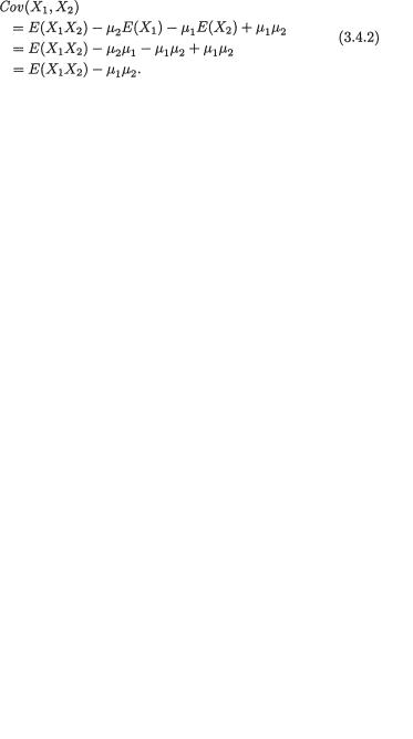
tion g(X1, X2) = (X1 – 1)(X2 – 2) of the two random variables X1, X2. By combining the ideas from (3.2.6) and (3.3.8) we can easily rewrite (3.4.1).
Then, using the Theorem 3.3.2 we obtain
We now rewrite (3.4.2) in its customary form, namely
whether X1, X2 are discrete or continuous random variables, provided that the expectations E(X1 X2), E(X1) and E(X2) are finite. From (3.4.3) it also becomes clear that
120 3. Multivariate Random Variables
where X1, X2 are any two arbitrary discrete or continuous random variables, that is the covariance measure is symmetric in the two variables. From (3.4.3) it obviously follows that
where X1 is any arbitrary random variable having a finite second moment.
Theorem 3.4.1 Suppose that Xi, Yi, i = 1, 2 are any discrete or continuous random variables. Then, we have
(i)Cov(X1, c) = 0 where c is fixed, if E(X1) is finite;
(ii)Cov(X1 + X2, Y1 + Y2) = Cov(X1, Y1) + Cov(X1, Y2) + Cov(X2, Y1) + Cov(X2, Y2) provided that Cov(Xi, Yj)
is finite for i, j = 1, 2.
In other words, the covariance is a bilinear operation which means that it is a linear operation in both coordinates.
Proof (i) Use (3.4.3) where we substitute X2 = c w.p.1. Then, E(X2) = c and hence we have
(ii) First let us evaluate Cov(X1 + X2, Y1). One gets
Next,
This leads to the final conclusion by appealing again to (3.4.4). ¢
3. Multivariate Random Variables |
121 |
Example 3.4.1 (Examples 3.2.4 and 3.2.5 Continued) We already know that E(X1) = 2.27 and also E(X1X2) = 3.05. Similarly, we can find E(X2) = (1)(.55) + 2(.45) = 1.45 and hence, Cov(X1, X2) = 3.05 – (2.27)(1.45) = – 0.2415. !
Example 3.4.2 (Example 3.3.3 Continued) It is easy to see that E(X1) =
(1/3)(1/2) = 1/6. Next, we appeal to (3.4.3) and observe that Cov(X1, X2) = E(X1X2) – E(X1)E(X2) = 1/6 – (1/3)(1/2) = 0. !
Example 3.4.3 (Example 3.3.5 Continued) It is easy to see that E(X1) =
peal to (3.4.3) and observe that Cov(X1, X2) = E(X1X2) – E(X1)E(X2) = 3/10 – (3/4)(3/8) = 3/160. !
The term Cov(X1, X2) can be any real number, positive, negative or zero. However, if we simply look at the value of Cov(X1, X2), it will be hard for us to say very much about the strength of the dependence between the two random variables X1 and X2 under consideration. It should be apparent that the term Cov(X1, X2) has the unit of measurement which is same as that for the variable X1X2, the product of X1 and X2. If X1, X2 are both measured in inches, then Cov(X1, X2) would have to be recorded in square inches.
A standardized version of the covariance term, commonly known as the correlation coefficient, was made popular by Karl Pearson. Refer to Stigler (1989) for the history of the invention of correlation. We discuss related historical matters later.
Definition 3.4.2 The correlation coefficient between any two random variables X1 and X2, denoted by ρX1, X2, is defined as follows:
whenever one has –∞ < Cov(X1, X2) < ∞, |
and |

122 3. Multivariate Random Variables
When we consider two random variables X1 and X2 only, we may supress the subscripts from ρX1, X2 and simply write ρ instead.
Definition 3.4.3 Two random variables X1, X2 are respectively called negatively correlated, uncorrelated, or positively correlated if and only if ρX1, X2 negative, zero or positive.
Before we explain the role of a correlation coefficient any further, let us state and prove the following result.
Theorem 3.4.2 Consider any two discrete or continuous random variables X1 and X2 for which we can assume that –∞ < Cov(X1, X2) < ∞, 0 < V(X1) < ∞ and 0 < V(X2) < ∞. Let ρX1, X2, defined by (3.4.8), stand for the correlation coefficient between X1 and X2. We have the following results:
(i)Let Yi = ci + diXi where –∞ < ci < ∞ and 0 < di < ∞ arefixed numbers, i = 1, 2. Then, ρY1,Y2 = ρX1, X2;
(ii)|ρX1, X2| ≤ 1;
(iii)In part (ii), the equality holds, that is ρ is +1 or –1, if and only
if X1 and X2 are linearly related. In other words, ρX1, X2 is +1or – 1 if and onlyif X1 = a + bX2 w.p.1 for some real numbers a and b.
Proof (i) We apply the Theorem 3.3.2 and Theorem 3.4.1 to claim that
Also, we have
Next we combine (3.4.8)-(3.4.10) to obtain
(ii) We apply the Cauchy-Schwarz inequality (Theorem 3.9.5) or directly the covariance inequality (Theorem 3.9.6) from the Section 3.9 and imme-

3. Multivariate Random Variables |
123 |
diately note that
From (3.4.12) we conclude that
Hence, one has |ρX1, X2| = 1.
|
(iii) We conclude that , |
X2 = 1 provided that we have equality throughout |
||
(3.4.13). The covariance inequality (Theorem 3.9.6) dictates that we can |
||||
have equality in (3.4.13) if and only if the two random variables (X |
– µ ) and |
|||
(X |
– µ ) are linearly related w.p.1. In other words, one will have , 1 |
1 |
= 1 |
|
2 |
2 |
|
X2 |
|
if and only if (X1 – µ1) = c(X2 – µ2) + d w.p.1 where c and d are two real numbers. The result follows with a = µ1 – cµ2 + d and b = c. One may observe that ρX1, X2 = +1 or –1 according as b is positive or negative. ¢
From the Definition 3.4.3, recall that in the case when ρX1, X2 = 0, the two random variables X1, X2 are called uncorrelated. The case of zero correlation is addressed in more detail in the Section 3.7.
If the correlation coefficient ρ is one in magnitude, then the two random variables are linearly related with probability one.
The zero correlation is referred to as uncorrelation.
Example 3.4.4 (Example 3.4.1 Continued) One can check that V(X1) = 6.4971 and V(X2) = .6825. We also found earlier that Cov(X1, X2) = –0.2415. Thus, using
(3.4.8) we get ρX1, X2 = Cov(X1, X2)/(σ1σ2) = ≈ –
. 11468. !
Example 3.4.5 (Example 3.4.2 Continued) We already had shown that Cov(X1, X2) = 0. One can also check that both V(X1) and V(X2) are finite, and hence ρX1, X2 = 0. !
Example 3.4.6 (Example 3.4.3 Continued) We already had shown that Cov(X1, X2) = 3/160 whereas E(X ) = 3/4, E(X ) = 3/8. Proceeding analogously, one can check that 
Thus, V(X1) = 3/5 – (3/4)2 = 3/80 and V(X2) = 1/5 – (3/8)2 = 19/320.
Hence, ρX1, X2 = (3/160) |
/ ≈ .39736. ! |

124 3. Multivariate Random Variables
Next, we summarize some more useful results for algebraic manipulations involving expectations, variances, and covariances.
Theorem 3.4.3 Let us write a1, ..., ak and b1, ..., bk for arbitrary but fixed real numbers. Also recall the arbitrary k-dimensional random variable X = (X1, ..., Xk) which may be discrete or continuous. Then, we have
Proof The parts (i) and (ii) follow immediately from the Theorem 3.3.2 and (3.4.3). The parts (iii) and (iv) follow by successively applying the bilinear property of the covariance operation stated precisely in the Theorem 3.4.1, part (ii). The details are left out as the Exercise 3.4.5. ¢
One will find an immediate application of Theorem 3.4.3 in a multinomial distribution.
3.4.1 The Multinomial Case
Recall the multinomial distribution introduced in the Section 3.2.2. Suppose that X = (X1, ..., Xk) has the Multk(n, p1, ..., pk) distribution with the associated pmf given by (3.2.8). We had mentioned that Xi has the Binomial(n, pi) distribution for all fixed i = 1, ..., k. How should we proceed to derive the expression of the covariance between Xi and Xj for all fixed i ≠ j = 1, ..., k?
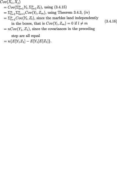
Recall the way we had motivated the multinomial pmf given by (3.2.8). Suppose that we have n marbles and these are tossed so that each marble lands in one of the k boxes. The probability that a marble lands in box #i is, say, pi, i = 1, ..., k,  Then, let Xl be the number of marbles landing in the box #l, l = i, j. Define
Then, utilizing (3.4.14) we can write
3. Multivariate Random Variables |
125 |
so that we have
It is not hard to see that E[Y1Z1] = 0, E[Y1] = pi, E[Z1] = pj, and hence we can rewrite (3.4.16) to claim that
for all fixed i ≠ j = 1, ..., k.
This negative covariance should intuitively make sense because out of the n marbles, large number of marbles in box #i would necessarily force the number of marbles in the box #j to be small. Next, one can simply obtain
for all fixed i ≠ j = 1, ..., k.
3.5 Independence of Random Variables
Suppose that we have a k-dimensional random variable X = (X1, ..., Xk) whose joint pmf or pdf is written as f(x) or f(x1, ..., xk) with xi χi( ), i = 1, ..., k. Here χi is the support of the random variable Xi, i = 1, ..., k, where these random variables can be discrete or continuous.
Definition 3.5.1 Let fi(xi) denote the marginal pmf or pdf of Xi, i = 1, ..., k. We say that X1, ..., Xk form a collection of independent random variables if and only if
126 3. Multivariate Random Variables
Also, X1, ..., Xk form a collection of dependent random variables if and only if these are not independent.
In order to show that X1, ..., Xk are dependent, one simply needs to show the existence of a particular set of values x1, ..., xk, with xi χi, i = 1, ..., k such that 
Example 3.5.1 (Example 3.2.4 Continued) We immediately note that P(X1
= –1 ∩ X2 = 1) = .12, P(X1 = –1) = .32 and P(X2 = 1) = .55. But, P(X1 = – 1)P(X2 = 1) = .176 which is different from P(X1 = –1 ∩ X2 = 1). We have
shown that when x1 = –1, x2 = 1 are chosen, then, f(x1,x2) ≠ f1(x1)f2(x2. Thus, the two random variables X1, X2 are dependent. !
Example 3.5.2 (Example 3.3.1 Continued) From (3.3.9)-(3.3.11) we have
f(x1, x2) = 6(1 – x2) for 0 < x1 < x2 < 1,  fi(xi) = 18x2(1 – x1)2(1 – x2) for 0 < x1, x2 < 1. For x1 = .4, x2 = .5, we have f(x1, x2) = 3, but
  fi(xi) = 1.62 ≠ f(x1, x2). Thus, the two random variables X1, x2 are dependent. !
Example 3.5.3 Consider two random variables X1, X2 having their joint pdf given by
First, one can easily show that fi(xi) = 2xi for 0 < xi < 1, i = 1, 2. Since one
obviously has f(x1, x2) = f1(x1) f2(x2) for all 0 < x1, x2 < 1, it follows that X1, X2 are independent. !
It is important to understand, for example, that in order for the k random variables X1, X2, ..., Xk to be independent, their joint and the marginal pmf’s or the pdf’s must satisfy (3.5.1).
Look at the next example for the case in point.
Example 3.5.4 It is easy to construct examples of random variables X1, X2, X3 such that (i) X1 and X2 are independent, (ii) X2 and X3 are independent, and (iii) X1 and X3 are also independent, but (iv) X1, X2, X3 together are dependent. Suppose that we start with the non-negative integrable functions fi(xi)
for 0 < xi < 1 which are not identically equal to unity such that we have 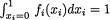 , i = 1, 2, 3. Let us then define
3. Multivariate Random Variables |
127 |
for 0 < xi < 1, i = 1, 2, 3. It is immediate to note that g(x1, x2, x3) is a bona fide pdf. Now, focus on the three dimensional random variable X = (X1, X2, X3) whose joint pdf is given by g(x1, x2, x3). The marginal pdf of the random variable Xi is given by gi(xi) = 1/2{fi(xi) + 1} for 0 < xi < 1, i = 1, 2, 3. Also the
joint pdf of (Xi, Xj) is given by gi, j(xi, xj) = 1/4{fi(xi)fj(xj) + fi(xi) + fj(xj) + 1} for i ≠ j = 1, 2, 3. Notice that gi, j(xi, xj) = gi(xi)gj(xj) for i ≠ j = 1, 2, 3, so that we
can conclude: Xi and Xj are independent for i ≠ j = 1, 2, 3. But, obviously g(x1, x2, x3) does not match with the expression of the product  for 0 < xi < 1, i = 1, 2, 3. Refer to the three Exercises 3.5.4-3.5.6 in this context.!
In the Exercises 3.5.7-3.5.8 and 3.5.17, we show ways to construct
afour-dimensional random vector X = (X1, X2, X3, X4) such that X1, X2, X3 are independent, but X1, X2, X3, X4 are dependent.
For a set of independent vector valued random variables X1, ..., Xp, not necessarily all of the same dimension, an important consequence is summarized by the following result.
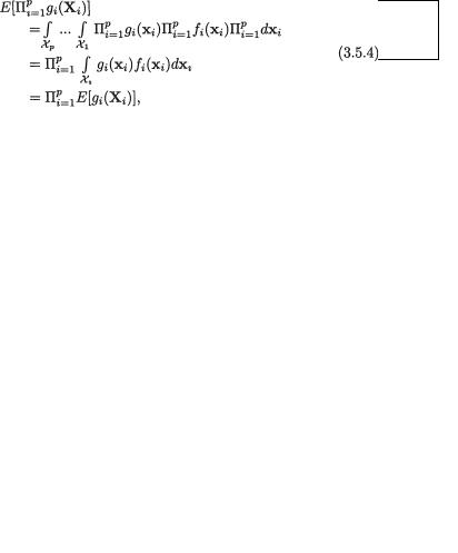
Theorem 3.5.1 Suppose that X1, ..., Xp are independent vector valued random variables. Consider real valued functions gi(xi), i = 1, ..., p. Then, we have
as long as E[gi(Xi)] is finite, where this expectation corresponds to the integral with respect to the marginal distribution of Xi, i = 1, ..., p. Here, the Xi’s may be discrete or continuous.
Proof Let the random vector Xi be of dimension ki and let its support be χiki, i = 1, ..., k. Since X1, ..., Xp are independent, their joint pmf or pdf is given by
Then, we have

128 3. Multivariate Random Variables
which is the desired result. ¢
One important consequence of this theorem is this: if two real valued random variables are independent, then their covariance, when finite, is necessarily zero. This in turn then implies that the correlation coefficient between those two random variables is indeed zero.
In other words, independence between the random variables X1 and X2 would lead to the zero correlation between X1 and X2 as long as ρ x1, x2 is finite. We state this more generally as follows.
Theorem 3.5.2 Suppose that X1, X2 are two independent vector valued random variables, not necessarily of the same dimension. Then,
(i)Cov(g1(X1),g2(X2)) = 0 where g1(.),g2(.) are real valued func tions, if E[g1g2], E[g1] and E[g2] are all finite;
(ii)g1(X1),g2(X2) are independent where g1(.),g2(.) do not need to be restricted as only real valued.
Proof (i) Let us assume that E[g1g2], E[g2] and E[g2] are all finite. Then, we appeal to the Theorem 3.5.1 to assert that E[g1(X1)g2(X2)] =
E[g1(X1)]E[g2(X2)]. But, since Cov(g1(X1), g2(X2)) is E[g1(X1)g2)] – E[g1(X1)]E[g2)], we thus have Cov(g1(X1,g2(X2)) obviously reducing to zero.
(ii) We give a sketch of the main ideas. Let Ai be any Borel set in the range space of the function gi(.), i = 1, 2. Now, let Bi = {xi χi : gi(xi) Ai}. Now,
which is the desired result. ¢
In the Theorem 3.5.2, one may be tempted to prove part (i) using the result from part (ii) plus the Theorem 3.5.1, and wonder whether the requirements of the finite moments stated therein are crucial for the
conclusion to hold. See the following example for the case in point.
Example 3.5.5 Suppose that X1 is distributed as the standard normal
variable with its pdf |
φ ( x1) defined in |
|||
(1.7.16) and X |
2 |
is distributed as the Cauchy variable with its pdf f (x ) = π–1 |
||
|
|
2 |
2 |
|
 defined in (1.7.31), –∞ < x1, x2 < ∞. Suppose also that

3. Multivariate Random Variables |
129 |
these two random variables are independent. But, we can not claim that Cov(X1, X2) = 0 because E[X2] is not finite. !
Two random variables X1 and X2 may be independent, but that may not necessarily imply that Cov(X1, X2) = 0.
This has been emphasized in the Example 3.5.5.
Example 3.5.6 What will happen to the conclusions in the Theorem 3.3.1, parts (i)-(ii), when the two random variables X1 and X2 are indepen-
dent? Let X1 and X2 be independent. Then, E2|1{X2 | X1} = E[X2] which is a constant, so that E1[E{X2}] = E[X2]. Also, V1[E2|1{X2 | X1}] = V1[E{X2}] = 0 since the variance of a constant is zero. On the other hand,
V[X2] which is a constant. Thus, E1[V2|1{X2 | X1}] = E1[V{X2}] = V[X2]. Hence, V1[E2|1{X2 | X1}] + E1[V2|1{X2 | X1}] simplifies to V[X2]. !
We have more to say on similar matters again in the Section 3.7. We end this section with yet another result which will come in very handy in verifying whether some jointly distributed random variables are independent. In some situations, applying the Definition 3.5.1 may be a little awkward because (3.5.1) requires one to check whether the joint pmf or the pdf is the same as the product of the marginal pmf’s or pdf’s. But, then one may not yet have identified all the marginal pmf’s or pdf’s explicitly! What is the way out? Look at the following result. Its proof is fairly routine and we leave it as the Exercise 3.5.9.
Suppose that we have the random variables X1, ..., Xk where χi is the support of Xi, i = 1, ..., k. Next, we formalize the notion of the supports χi’s being unrelated to each other.
Definition 3.5.2 We say that the supports χi’s are unrelated to each other if the following condition holds: Consider any subset of the random variables, Xij, j = 1, ..., p, p = 1, ..., k – 1. Conditionally, given that Xij = xij, the support of the remaining random variable Xl stays the same as χl for any l ≠ ij, j = 1,
..., p, p = 1, ..., k – 1.
Theorem 3.5.3 Suppose that the random variables X1, ..., Xk have the joint pmf or pdf f(x1, ..., xk), xi χl, the support of Xi, i = 1, ..., k. Assume that these supports are unrelated to each other according to the Definition 3.5.2. Then, X1, ..., Xk are independent if and only if
for some functions h1(x1), ..., hk(xk).
130 3. Multivariate Random Variables
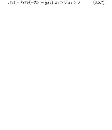
Example 3.5.7 Suppose that the joint pdf of X1, X2 is given by
for some θ > 0 where k(> 0) is a constant. Obviously, we can write f(x1, x2) =
kh1(x1)h2(x2) for all positive numbers x1, x2 where h1(x1) = exp{–θx1} and h2(x2) = exp{–1/θx2}. Also the supports χ1 = +, χ2 = + are unrelated to each other.
Hence, by appealing to the Theorem 3.5.3 we can claim that X1 and X2 are independent random variables. One should note two interesting facts here. The two chosen functions h1(x1) and h2(x2) are not even probability densities to begin with. The other point is that the choices of these two functions are not unique. One can easily replace these by kdh1(x1) and kd–1h2(x2) respectively where d(> 0) is any arbitrary number. Note that we did not have to determine k in order to reach our conclusion that X1 and X2 are independent random variables. !
Example 3.5.8 (Example 3.5.7 Continued) One can check that f1(x1) = θ exp{–θx1} and f2(x2) = θ–1exp{–1/θ . x2}, and then one may apply (3.5.1) instead to arrive at the same conclusion. In view of the Theorem 3.5.3 it becomes really simple to write down the marginal pdf’s in the case of independence. !
Example 3.5.9 Suppose that the joint pdf of X1, X2, X3 is given by
where c(> 0) is a constant. One has f(x1, x2, x3) = ch1(x1)h2(x2)h3(x3) with
 exp{–2x1}, and h3(x3) = exp
 , for all values of x1 +, (x2, x3) Î 2. Also, the supports χ1 +, χ2 = , χ3 = are unrelated to each other. Hence, by appealing to the Theorem 3.5.3 we
can claim that X1, X2 and X3 are independent random variables. One should again note the interesting facts. The three chosen functions h1(x1), h2(x2) and h3(x3) are not even probability densities to begin with. The other point is that the choices of these three functions are not unique. !
Example 3.5.10 (Example 3.5.9 Continued) One should check these out: By looking at h1(x1) one can immediately guess that X1 has the Gamma(α = 1/2, β = 1/2) distribution so that its normalizing constant  . By looking at h2(x2) one can immediately guess that X2 has the Cauchy distribution so that its normalizing constant 1/π. Similarly, by looking at h3(x3) one can immediately guess that X3 has the N(0, 1/2π) distribution so that its normalizing constant is unity. Hence,
  (1/π)(1)=

3. Multivariate Random Variables |
131 |
Refer to (1.7.13), (1.7.20) and (1.7.31) as needed. Note that the Theorem 3.5.3 really makes it simple to write down the marginal pdf’s in the case of independence. !
It is crucial to note that the supports χi’s are assumed to be unrelated to each other so that the representation given by (3.5.6) may lead to the conclusion of independence among the random variables Xi’s. Look at the Example 3.5.11
to see what may happen when the supports are related.
Example 3.5.11 (Examples 3.3.1 and 3.5.2 Continued) Consider two random variables X1 and X2 whose joint continuous distribution is given by the following pdf:
Obviously, one has χ1 = χ2 = (0, 1). One may be tempted to denote, for example, h1(x1) = 6, h2(x2) = (1 – x2). At this point, one may be tempted to claim that X1 and X2 are independent. But, that will be wrong! On the whole space χ1 × χ2, one can not claim that f(x1, x2) = h1(x1)h2(x2). One may check this out by simply taking, for example, x1 = 1/2, x2 = 1/4 and then one has f(x1, x2) = 0 whereas h1(x1)h2(x2) = 9/2. But, of course the relationship f(x1, x2) = h1(x1)h2(x2) holds in the subspace where 0 < x1 < x2 < 1. From the Example 3.5.2 one will recall that we had verified that in fact the two random variables X1 and X2 were dependent. !
3.6 The Bivariate Normal Distribution
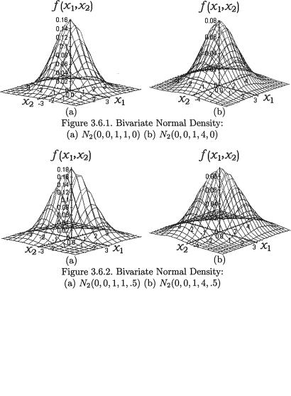
Let (X1, X2) be a two-dimensional continuous random variable with the following joint pdf:
with
The pdf given by (3.6.1) is known as the bivariate normal or two-dimensional normal density. Here, µ1, µ2, σ1, σ2 and ρ are referred to as the parameters
132 3. Multivariate Random Variables
of the distribution. A random variable (X1, X2) having the pdf given by (3.6.1) is denoted by N2(µ1, µ2,  , ρ). The pdf f(x1, x2) from (3.6.1) is centered around the point (µ1, µ2) in the x1, x2 plane. The bivariate normal pdf given by (3.6.1) has been plotted in the Figures 3.6.1-3.6.2.
The Figure 3.6.2 (a) appears more concentrated around its center than its counterpart in the Figure 3.6.1 (a). This is due to the fact that we have taken ρ = .5 to draw the former picture in contrast with the value ρ = 0 in the latter picture, while the other parameters are held fixed. Clearly, the ordinate at the center in the Figure 3.6.1 (a) happens to be 1/2π (≈ .15915) whereas the ordinate at the center in the Figure 3.6.2 (a) happens to be (1/ 2π) (≈ .18378) which is larger. This justifies the preceding claim. One observes a similar feature when the Figures 3.6.1 (b)-3.6.2 (b)
3. Multivariate Random Variables |
133 |
are visually compared.
How can one show directly that f(x1, x2) from (3.6.1) is indeed a genuine pdf? The derivation follows shortly.
The function f(x1, x2) is always positive. So, we merely need to verify that the double integral of f(x1, x2) over the whole space 2 is unity. With u1, u2 from (3.6.2), let us then rewrite
Hence, with c defined in (3.6.2) we obtain
Now, for all fixed x2 , let us denote
so that with |
we obtain |
Next, look at the expression of ag(x1, x2) obtained from (3.6.5) and note that for all fixed x2, it resembles the pdf of a univariate normal variable with mean µ1 + ρσ1(x2 – µ2)/σ2 and variance  at the point x1 . Hence, we must have
134 3. Multivariate Random Variables
Again note that with  , the expression bh(x2) obtained from (3.6.5) happens to be the pdf of a normal variable with mean µ2 and variance
  at the point x2 . Hence, we must have
so that (3.6.8) can be rewritten as
by the definition of c from (3.6.2). Thus, we have directly verified that the function f(x1, x2) given by (3.6.1) is indeed a genuine pdf of a two-dimen- sional random variable with its support 2.
Theorem 3.6.1 Suppose that (X1, X2) has the N2 (µ1, µ2,  , ρ) distribution with its pdf f(x1, x2) given by (3.6.1). Then,
(i)the marginal distribution of Xi is given by N(µi,  ), i = 1, 2;
(ii)the conditional distribution of X1 | X2 = x2 is normal with mean
µ1+ (x2 – µ2) and variance ), |
for all |
|
fixed x2 ; |
|
|
(iii) the conditional distribution of X2 | X1 = x1 is normal with |
||
x .µ2 + |
(x1 – µ1) and variance |
, for all fixed |
1 |
|
|
Proof (i) We simply show the derivation of the marginal pdf of the random variable X2. Using (3.3.2) one gets for any fixed x2 ,
which can be expressed as
This shows that X2 is distributed as N(µ2,  ). The marginal pdf of X1 can be found easily by appropriately modifying (3.6.5) first. We leave this as the Exercise 3.6.1.

3. Multivariate Random Variables |
135 |
(ii) Let us denote  and a = {2π(1–
. Utilizing (3.3.5), (3.6.4)-(3.6.5) and (3.6.11), the conditional pdf of X1 | X2 = x2 is given by
The expression of f1|2(x1) found in the last step in (3.6.12) resembles the pdf of a normal random variable with mean  and variance
(iii) Its proof is left as the Exercise 3.6.2. ¢
Example 3.6.1 Suppose that (X1, X2) is distributed as N2 (0,0,4,1,ρ) where ρ = 1/2. From the Theorem 3.6.1 (i) we already know that E[X2] = 0 and V[X2] = 1. Utilizing part (iii), we can also say that E[X2 | X1 = x1] = 1/4x1 and V[X2 | X1 = x1] = 3/4. Now, one may apply the Theorem 3.3.1 to find indirectly the expressions of E[X2] and V[X2]. We should have E[X2] = E{E[X2 |
X1 = x1]} = E[1/4 X1] = 0, whereas V[X2] = V{E[X2 | X1 = x1]} + E{V[X2 | X1 = x1]} = V[1/4X1] + E[3/4] = 1/16V[X1] + 3/4 = 1/16(4) + 3/4 = 1. Note that
in this example, we did not fully exploit the form of the conditional distribution of X2 | X1 = x1. We merely used the expressions of the conditional mean and variance of X2 | X1 = x1. !
In the Example 3.6.2, we exploit more fully the form of the conditional distributions.
Example 3.6.2 Suppose that (X1, X2) is distributed as N2(0,0,1,1,ρ) where ρ = 1/2. We wish to evaluate E{exp[1/2X1X2]}. Using the Theorem 3.3.1 (i), we can write
But, from the Theorem 3.6.1 (iii) we already know that the conditional distribution of X2 | X1 = x1 is normal with mean 1/2x1 and variance 3/4. Now, E(exp1/2x1X2] | X1 = x1) can be viewed as the conditional mgf of X2 | X1 = x1. Thus, using the form of the mgf of a univariate normal random variable from (2.3.16), we obtain
136 3. Multivariate Random Variables
From the Theorem 3.6.1 (i), we also know that marginally X1 is distributed as N(0,1). Thus, we combine (3.6.13)-(3.6.14) and get
With σ2 = 16/5, let us denote  exp{–5/32u2}, u . Then, h(u) is the pdf of a random variable having the N(0,σ2) distribution so that ∫ h(u)du = 1. Hence, from (3.6.15) we have
In the same fashion one can also derive the mgf of the random variable
X1X2, that is the expression for the E{exp[tX1X2]} for some appropriate range of values of t. We leave this as the Exercise 3.6.3. !
The reverse of the conclusion given in the Theorem 3.6.1, part (i) is not necessarily true. That is, the marginal distributions of both X1 and X2 can be univariate normal, but this does not imply that (X1,X2) is jointly distributed as N2. Look at the next example.
Example 3.6.3 In the bivariate normal distribution (3.6.1), each random variable X1,X2 individually has a normal distribution. But, it is easy to construct two dependent continuous random variables X1 and X2 such that marginally each is normally distributed whereas jointly (X1,X2) is not distributed as N2.
Let us temporarily write f(x1, x2;µ1,µ2, ρ) for the pdf given in (3.6.1). Next, consider any arbitrary 0 < α , ρ < 1 and fix them. Let us now define
for–∞ < x1, x2 < ∞ f(x1, x2; 0, 0, 1, 1, –
Since the non-negative functions f(x1, x2; 0,0,1,1,ρ) and ρ) are both pdf’s on 2, we must have

3. Multivariate Random Variables |
137 |
Hence, we can express ∫ 2∫ g(x1, x2; ρ) dx1 dx2 as
Also, g(x1, x2;ρ) is non-negative for all (x1, x2) 2. Thus, g(x1, x2) is a genuine pdf on the support 2.
Let (X1, X2) be the random variables whose joint pdf is g(x1, x2;ρ) for all (x1, x2) 2. By direct integration, one can verify that marginally, both X1 and X2 are indeed distributed as the standard normal variables.
The joint pdf g(x1, x2; ρ) has been plotted in the Figures 3.6.3 (a) and (b) with α = .5,.1 respectively and α = .5. Comparing these figures visually with those plotted in the Figures 3.6.1-3.6.2, one may start wondering whether g(x1, x2; ρ) may correspond to some bivariate normal pdf after all!
Figure 3.6.3. The PDF g(x1, x2; ρ) from (3.6.17):
(a) ρ = .5, α = .5 (b) ρ = .5, α = .1
But, the fact of the matter is that the joint pdf g(x1, x2; ρ) from (3.6.17) does not quite match with the pdf of any bivariate normal distribution. Look at the next example for some explanations. !
How can one prove that the joint pdf g(x1, x2;ρ) from (3.6.17) can not match with the pdf of any bivariate normal distribution?
Look at the Example 3.6.4.
Example 3.6.4 (Example 3.6.3 Continued) Consider, for example, the situation when ρ = .5, α = .5. Using the Theorem 3.6.1 (ii), one can check

138 3. Multivariate Random Variables
that
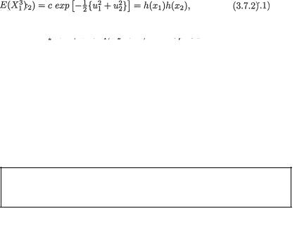
whatever be fixed x2 , since α = .5. Suppose that it is possible for the pair (X1, X2) to be distributed as the bivariate normal variable, N2(0,0,1,1, ρ*) with some ρ* (–1, 1). But, then E[X1 | X2 = x2] must be ρ*x2 which has to match with the answer zero obtained in (3.6.19), for all x2 . In other words, ρ* must be zero. Hence, for all (x1, x2) 2 we should be able to write
Now, g(0,0; ρ = .5) =  , but h(0,0) = 1/2π. It is obvious that g(0,0; π =.5)
≠ h(0,0). Hence, it is impossible for the random vector (X1, X2) having the pdf g(x1, x2; ρ = .5) to be matched with any bivariate normal random vector. !
The Exercise 3.6.8 gives another pair of random variables X1 and X2 such that marginally each is normally distributed whereas jointly (X1, X2) is not distributed as N2.
For the sake of completeness, we now formally define what is known as the regression function in statistics.
Definition 3.6.1 Suppose that (X1, X2) has the N2 (µ1, µ2,  , ρ) distribution with its pdf f(x1, x2) given by (3.6.1). The conditional mean of X1 | X2 = x2, that is, µ1 + (x2–µ2) is known as the regression function of X1 on X2. Analogously, the conditional mean of X2 | X1 = x1, that is, µ2 +
  (x1 – µ1) is known as the regression function of X2 on X1.
Even though linear regression analysis is out of scope for this textbook, we simply mention that it plays a very important role in statistics. The readers have already noted that the regression functions in the case of a bivariate normal distribution turn out to be straight lines.
We also mention that Tong (1990) had written a whole book devoted entirely to the multivariate normal distribution. It is a very valuable resource, particularly because it includes the associated tables for the percentage points of the distribution.
3. Multivariate Random Variables |
139 |
3.7 Correlation Coefficient and Independence
We begin this section with a result which clarifies the role of the zero correlation in a bivariate normal distribution.
Theorem 3.7.1 Suppose that (X1, X2) has the bivariate normal distribution N2(µ1, µ2,  , ρ) with the joint pdf given by (3.6.1) where –∞
< µ1, µ2 < ∞, 0 < σ1, σ2 < ∞ and –1 < ρ < 1. Then, the two random variables X1 and X2 are independent if and only if the correlation coeffi-
cient ρ = 0.
Proof We first verify the “necessary part” followed by the “sufficiency part”.
Only if part: Suppose that X1 and X2 are independent. Then, in view of the Theorem 3.5.2 (i), we conclude that Cov(X1, X2) = 0. This will imply that ρ = 0.
If part: From (3.6.1), let us recall that the joint pdf of (X1, X2) is given
by
with
But, when ρ = 0, this joint pdf reduces to
where  exp{–1/2(xi – i)2/
  }, i = 1, 2. By appealing to the Theorem 3.5.3 we conclude that X1 and X2 are independent. ¢
However, the zero correlation coefficient between two arbitrary random variables does not necessarily imply that these two variables are independent. Examples 3.7.1-3.7.2 emphasize this point.
Example 3.7.1 Suppose that X1 is N(0, 1) and let `X2 =  . Then,
Cov(X1, X2) = E(X1X2) – E(X1)E(X2) =  – E(X1)E(X2) = 0, since E(X1) = 0 and = 0. That is, the correlation coefficient ρX1,X2 is
zero. But the fact that X1 and X2 are dependent can be easily verified as follows. One can claim that P {X2 > 4} > 0, however, the conditional probability, P {X2 > 4 | –2 ≤ X1 ≤ 2} is same as P  –2 ≤ X1 ≤ 2}

140 3. Multivariate Random Variables
which happens to be zero. Thus, we note that P {X2 > 4 | –2 ≤ X1 ≤ 2} ≠ P {X2 > 4}. Hence, X1 and X2 are dependent variables. !
One can easily construct similar examples in a discrete situation. Look at the Exercises 3.7.1-3.7.3.
Example 3.7.2 Suppose that Θ is distributed uniformly on the interval [0, 2π). Let us denote X1 = cos(Θ), X2 = sin(Θ). Now, one has E[X1] =  Also, one can write E[X1X2] =
  Thus,
Thus,
Cov(X1, X2) = E(X1X2) – E(X1)E(X2) = 0 – 0 = 0. That is, the correlation coefficient ρX1,X2 is zero. But the fact that X1 and X2 are dependent can be
easily verified as follows. One observes that  and hence conditionally given X1 = x1, the random variable X2 can take one of the possible values, or
  with probability 1/2 each. Suppose that we fix x1 = . Then, we argue that P{–1/4 < X2 < 1/4 | X1 =
  } = 0, but obviously P{–1/4 < X2 < 1/4} > 0. So, the random variables X1 and X2 are dependent. !
Theorem 3.7.1 mentions that ρX1,X2 = 0 implies independence between X1 and X2 when their joint distribution is N2. But, ρX1,X2 = 0 may sometimes imply independence between
X1 and X2 even when their joint distribution is different from the bivariate normal. Look at the Example 3.7.3.
Example 3.7.3 The zero correlation coefficient implies independence not merely in the case of a bivariate normal distribution. Consider two random variables X1 and X2 whose joint probability distribution is given as follows: Each expression in the Table 3.7.1 involving the p’s is assumed positive and smaller than unity.
Table 3.7.1. Joint Probability Distribution of X1 and X2
|
0 |
X1values |
1 |
Row |
|
|
Total |
||
0 |
|
|
|
|
1 – p1 |
p1+ p |
1 – p2 |
|
|
X2 |
– p1 +p |
|
|
|
values |
|
|
|
|
1 |
p2 – p |
|
p |
p2 |
Col. Total |
|
|
|
1 |
1 – p1 |
|
p1 |
Now, we have Cov(X1, X2) = E(X1X2)–E(X1)E(X2) = P{X1 = 1∩X2 = 1} – P{X1 = 1} P{X2 = 1} = p – p1p2, and hence the zero correlation
3. Multivariate Random Variables |
141 |
coefficient between X1 and X2 will amount to saying that p = p1p2 where so far p, p1 and p2 have all been assumed to lie between (0, 1) but they are otherwise arbitrary. Now, we must have then P(X1 = 1∩X2 = 0) = p1 – p, and P(X1 =
0nX2 = 0) = 1–p1–p2+p, and P(X1=0∩X2=1) = p2–p. But, now P(X1 = 0nX2 = 1) = p2–p = p2–p1p2 = p2(1–p1) = P(X1=0) P(X2=1); P(X1 = 1 ∩ X2 = 0) = p1 – p = p1 – p1p2 = p1(1 – p2) = P(X1 = 1) P(X2 = 0); and P(X1=0 ∩ X2=0) = 1–p1– p2+p = 1–p1–p2+p1p2 = (1–p1)(1–p2) = P(X1=0) P(X2=0). Hence, the two such random variables X1 and X2 are independent. Here, the zero correlation coef-
ficient implied independence, in other words the property that “the zero correlation coefficient implies independence” is not a unique characteristic property of a bivariate normal distribution. !
Example 3.7.4 There are other simple ways to construct a pair of random variables with the zero correlation coefficient. Start with two random vari-
ables U1, U2 such that V(U1) = V(U2). Let us denote X1 = U1 + U2 and X2 = U1
– U2. Then, use the bilinear property of the covariance function which says that the covariance function is linear in both components. This property was stated in the Theorem 3.4.3, part (iv). Hence, Cov(X1, X2) = Cov(U1 + U2, U1
– U2) = Cov(U1, U1) – Cov(U1, U2) + Cov(U2, U1) – Cov(U2, U2) = V(U1) –
V(U2) = 0. !
3.8 The Exponential Family of Distributions
The exponential family of distributions happens to be very rich when it comes to statistical modeling of datasets in practice. The distributions belonging to this family enjoy many interesting properties which often attract investigators toward specific members of this family in order to pursue statistical studies. Some of those properties and underlying data reduction principles, such as sufficiency or minimal sufficiency, would impact significantly in Chapter 6 and others. To get an idea, one may simply glance at the broad ranging results stated as Theorems 6.2.2, 6.3.3 and 6.3.4 in Chapter 6. In this section, we discuss briefly both the one-parameter and multi-parameter exponential families of distributions.
3.8.1 One-parameter Situation
Let X be a random variable with the pmf or pdf given by f(x; θ), x χ , θ Θ . Here, θ is the single parameter involved in the expression of f(x; θ) which is frequently referred to as a statistical model.

142 3. Multivariate Random Variables
Definition 3.8.1 We say that f(x;θ) belongs to the one-parameter exponential family if and only if we can express
with appropriate forms of real valued functions a(θ) ≥ 0, b(θ), g(x) ≥ 0 and R(x), where χ and Θ is a subinterval of the real line . It is crucial to note that the expressions of a(θ) and b(θ) can not involve x, while the expressions of g(x) and R(x) can not involve θ.
Many standard distributions, including several listed in Section 1.7, belong to this rich class. Let us look at some examples.
Example 3.8.1 Consider the Bernoulli distribution from (1.7.1). Let us rewrite the pmf f(x; p) as
which now resembles (3.8.1) where θ = p, a(θ) = 1 – θ, g(x) = 1, b(θ) = log{θ(1 – θ)–1}, R(x) = x, and Θ = (0, 1), χ = {0, 1}. !
Example 3.8.2 Let X be distributed as Poisson(λ), defined in (1.7.4) where λ(> 0). With χ = {0, 1, 2, ...}, θ = λ, and Θ = (0, ∞), the pmf f(x; θ) = e–θ θx/ x! has the same representation given in (3.8.1) where g(x) = (x!)–1, a(θ) = exp{–θ}, b(θ) = log(θ) and R(x) = x. !
Example 3.8.3 Let X be distributed as N(µ, 1), defined in (1.7.13) where µ . With χ = , θ = µ, and Θ = , the pdf  exp{– 1/2(x – θ)2} has the same representation given in (3.8.1) where g(x) = exp{– 1/2x2},
  exp{–1/2θ2}, b(θ) = θ and R(x) = x. !
One should not however expect that every possible distribution would necessarily belong to this one-parameter exponential family. There are many examples where the pmf or the pdf does not belong to the class of distributions defined via (3.8.1).
All one-parameter distributions do not necessarily belong to the exponential family (3.8.1). Refer to the Examples 3.8.4-3.8.6.
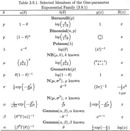
In the Table 3.8.1, we explicitly show the correspondence between some of the standard distributions mentioned in Section 1.7 and the associated representations showing their memberships in the one-parameter exponential family. While verifying the entries given in the Table 3.8.1, the reader will immediately realize that the expressions for a(θ), b(θ), g(x) and R(x) are not really unique.
3. Multivariate Random Variables |
143 |
Example 3.8.4 Consider a random variable X having a negative exponential pdf, defined in (1.7.36). The pdf is θ–1 exp{–(x – θ)/θ}I(x > θ) with θ > 0, where I(.) is an indicator function. Recall that I(A) is 1 or 0 according as the set A or Ac is observed. The term I(x > θ) can not be absorbed in the expressions for a(θ), b(θ), g(x) or R(x), and hence this distribution does not belong to a one-parameter exponential family. !
Example 3.8.5 Suppose that a random variable X has the uniform distribution, defined in (1.7.12), on the interval (0, θ) with θ > 0. The pdf can be rewritten as f(x; θ) = θ–1I(0 < x < θ). Again, the term I(x > θ) can not be absorbed in the expressions for a(θ), b(θ), g(x) or R(x), and hence this distribution does not belong to a one-parameter exponential family. !
144 3. Multivariate Random Variables
In the two Examples 3.8.4-3.8.5, the support χ depended on the single parameter θ. But, even if the support χ does not depend on θ, in some cases the pmf or the pdf may not belong to the exponential family defined via (3.8.1).
Example 3.8.6 Suppose that a random variable X has the N(θ, θ2) distribution where θ(> 0) is the single parameter. The corresponding pdf f(x; θ) can be expressed as
which does not have the same form as in (3.8.1). In other words, this distribution does not belong to a one-parameter exponential family. !
A distribution such as N(θ, θ2) with θ(> 0) is said to belong to a curved exponential family, introduced by Efron (1975, 1978).
3.8.2 Multi-parameter Situation
Let X be a random variable with the pmf or pdf given by f(x; θ), x χ , θ = (θ1, ..., θk) Θ k. Here, θ is a vector valued parameter having k components involved in the expression of f(x; θ) which is again referred to as a statistical model.
Definition 3.8.2 We say that f(x; θ) belongs to the k-parameter exponential family if and only if one can express
with some appropriate forms for g(x) ≥ 0, a(θ) ≥ 0, bi(θ) and Ri(x), i = 1, ..., k. It is crucial to note that the expressions of a(θ) and bi(θ), i = 1, ..., k, can not involve x, while the expressions of g(x) and R1(x), ..., Rk(x) can not involve θ.
Many standard distributions, including several listed in Section 1.7, belong to this rich class. In order to involve only statistically meaningful reparameterizations while representing f(x; θ) in the form given by (3.8.4), one would assume that the following regulatory conditions are satisfied:

3. Multivariate Random Variables |
145 |
In the contexts of both the one-parameter and multi-parameter exponential families, there are such notions referred to as the natural parameterization, the natural parameter space, and the natural exponential family. A serious discussion of these topics needs substantial mathematical depth beyond the assumed prerequisites. Elaborate discussions of intricate issues and related references are included in Chapter 2 of both Lehmann (1983, 1986) and Lehmann and Casella (1998), as well as Barndorff-Nielson (1978). Let us again consider some examples.
Example 3.8.7 Let X be distributed as N(µ, σ2), with k = 2, θ = (µ, σ)× + where µ and σ are both treated as parameters. Then, the correspond-
ing pdf has the form given in (3.8.4) where x , θ1 = µ, θ2 = σ, R1(x) = x,
R2(x) = x2, and  g(x) = 1,
  , and .
  !
!
Example 3.8.8 Let X be distributed as Gamma(α, β) where both α(> 0) and β (> 0) are treated as parameters. The pdf of X is given by (1.7.20) so that f(x; α, β) = {βα Γ(α)}–1exp(–x/β)xα–1, where we have k = 2, θ = (α, β)+ × +, x +. We leave it as an exercise to verify that this pdf is also of the form given in (3.8.4). !
The regularity conditions stated in (3.8.5) may sound too mathematical. But, the major consolation is that many standard and useful distributions in statistics belong to the exponential family and that the mathematical conditions stated in (3.8.5) are routinely satisfied.
3.9 Some Standard Probability Inequalities
In this section, we develop some inequalities which are frequently encountered in statistics. The introduction to each inequality is followed by a few examples. These inequalities apply to both discrete and continuous random variables.
3.9.1 Markov and Bernstein-Chernoff Inequalities
Theorem 3.9.1 (Markov Inequality) Suppose that W is a real valued random variable such that P(W = 0) = 1 and E(W) is finite. Then, for any fixed δ (> 0), one has:
Proof Suppose that the event A stands for the set [W ≥ δ], and then
146 3. Multivariate Random Variables
we can write
where recall that IA is the indicator function of A. One can check the validity of (3.9.2) as follows. On the set A, since one has IA = 1, the rhs of (3.9.2) is ä and it is true then that W ≥ δ. On the set Ac, however, one has IA = 0, so that the rhs of (3.9.2) is zero, but we have assumed that W ≥ 0 w.p.1. Next, observe that IA is a Bernoulli random variable with p = P(A). Refer to the Example 2.2.3 as needed. Since, W – δIA ≥ 0 w.p.1, we have E(W – δIA) = 0.
But, E(W – δIA) = E(W) – δP(A) so that E(W) – δP(A) = 0, which implies that P(A) ≥ δ–1 E(W). ¢
Example 3.9.1 Suppose that X is distributed as Poisson(λ = 2). From the Markov inequality, we can claim, for example, that P{X ≥ 1} ≤ (1)(2) = 2. But this bound is useless because we know that P{X ≥ 1} lies between 0 and 1. Also, the Markov inequality implies that P{X ≥ 2} ≤ (1/2)(2) = 1, which is again a useless bound. Similarly, the Markov inequality implies that P{X = 10} = (1/10)(2) = .2, whereas the true probability, P{X ≥ 10} = 1 – .99995 =
.00005. There is a serious discrepancy between the actual value of P{X ≥ 10} and its upper bound. However, this discussion may not be very fair because after all the Markov inequality provides an upper bound for P(W ≥ δ) without assuming much about the exact distribution of W. !
Example 3.9.2 Consider a random variable with its distribution as follows:
One may observe that E[X] = (–1/7)(.7)+(1)(.1)+(10)(.2) = 2 and P{X ≥ 10} = .2. In this case, the upper bound for P{X ≥ 10} obtained from (3.9.1) is also .2, which happens to match with the exact value of P{X ≥ 10}. But, that should not be the key issue. The point is this: The upper bound provided by the Markov inequality is distribution-free so that it works for a broad range of unspecified distributions. !
Note that the upper bound for P(W ≥ δ) given by (3.9.1) is useful only when it is smaller than unity.
The upper bound given by (3.9.1) may appear crude, but even so, the Markov inequality will work like a charm in some derivations.
The next Theorem 3.9.2 highlights one such application.
Theorem 3.9.2 (Bernstein-Chernoff Inequality) Suppose that X is a real valued random variable whose mgf Mx (t) is finite for some t T
3. Multivariate Random Variables |
147 |
(0, ∞). Then, for any fixed real number a, one has
Proof Observe that for any fixed t > 0, the three sets [X ≥ a], [tX ≥ ta] and [etX ≥ eta] are equivalent. Hence, for t Γ, we can rewrite P{X ≥ a} as
using (3.9.1) with W = etX, δ = eta. Now, since we are looking for an upper bound, it makes sense to pick the smallest upper bound available in this class. Thus, we take  as the upper bound. ¢
Example 3.9.3 Suppose that the random variable X has the exponential distribution with its pdf f(x) = e–xI(x > 0). The corresponding mgf is given by MX(t) = (1 – t)–1 for t e = (–∞, 1). For any fixed a > 1, the Theorem 3.9.2 implies the following:
Now, let us denote g(t) = e–ta(1 – t)–1 and h(t) = log(g(t)) for 0 < t < 1. It is easy to check that h’(t) = –a + (1 – t)–1, h’’(t) = (1 – t)–2 so that h’(t) = 0 when t ≡ t0 = 1 – a–1 which belongs to (0, 1). Also, h’’(t0) is positive so that the function h(t) attains the minimum at the point t = t0. Refer to (1.6.27) as needed. Since g(t) is a one-to-one monotone function of h(t), we conclude that the function g(t) attains the minimum at the point t = t0. In other words, we can rewrite (3.9.5) as
Does the upper bound in (3.9.6) lie between 0 and 1? In order to answer this question, next look at the function m(x) = (x – 1) – log(x) for x ≥ 1. Obviously, m(1) = 0 and m’(x) = 1 – x–1 ≥ 0, where equality holds if and only if x
=1. That is, for all x > 1, we have an increasing function m(x) But, since m(1)
=0, we claim that m(x) > 0 for x > 1. In other words, for a > 1, we have log(a) < a – 1 so that a < ea–1. Hence, the upper bound given by (3.9.6) is a number which lies between zero and one. !
The types of bounds given by (3.9.5) are customarily used in studying the rate of convergence of tail area probabilities.
148 3. Multivariate Random Variables
Example 3.9.4 Suppose that X is a random variable whose mgf MX(t) is finite for some t T (–∞, 0). Then, it follows from the Theorem 3.9.2 that for any fixed real number a, one can claim:
{e–ta MX(t)}. Its verification is left as the Exercise 3.9.1. !
The following section provides yet another application of the Markov inequality.
3.9.2 Tchebysheff’s Inequality
This inequality follows from a more general inequality (Theorem 3.9.4) which is stated and proved a little later. We take the liberty to state the simpler version separately for its obvious prominence in the statistical literature.
Theorem 3.9.3 (Tchebysheff’s Inequality) Suppose that X is a real valued random variable with the finite second moment. Let us denote its mean ì and variance α 2(> 0). Then, for any fixed real number ε(> 0), one has
We know that P{|X – µ| < kσ} = 1 – P{|X – µ| ≥ kσ}. Thus, with k > 0, if we substitute ε = kσ in (3.9.7), we can immediately conclude:
In statistics, sometimes (3.9.8) is also referred to as the Tchebysheff’s inequality. Suppose we denote pk = P{|X – µ| < kσ}. Again, (3.9.7) or equivalently (3.9.8) provide distribution-free bounds for some appropriate probability. Yet, let us look at the following table:
Table 3.9.1. Values of pk and the Tchebysheff’s Lower Bound (3.9.8)
|
k = 1 |
k = 2 |
k = 3 |
k = 4 |
Tchebysheff’s Bound |
0 |
3/4= .75 |
8/9 ≈ .88889 |
15/16 = .9375 |
pk: X is N(0, 1) |
.68268 |
.95450 |
.99730 |
.99994 |
|
|
|
|
|
In the case of the standard normal distribution, the Tchebysheff’s lower bound for pk appears quite reasonable for k = 3, 4. In the case k = 1, the Tchebysheff’s inequality provides a trivial bound whatever be the distribution of X.
3. Multivariate Random Variables |
149 |
Theorem 3.9.4 Suppose that X is a real valued random variable such that with some r > 0 and T T( ), one has ør = E{|X – T|r} which is finite. Then, for any fixed real number ε(> 0), one has
Proof Note that P{|X – T| ≥ ε} = P{W ≥ εr} where W = |X – T|r. Now, the inequality (3.9.9) follows immediately by invoking the Markov inequality. ¢
The Tchebysheff’s inequality follows immediately from (3.9.9) by substituting r = 2 and T = µ.
3.9.3 Cauchy-Schwarz and Covariance Inequalities
If we have independent random variables X1 and X2, then we know from the Theorem 3.5.1 that E[X1X2] = E[X1]E[X2]. But, if X1 and X2 are dependent, then it is not always so simple to evaluate E[X1X2]. The Cauchy-Schwarz inequality allows us to split E[X1X2] in the form of an upper bound having two separate parts, one involving only X1 and the other involving only X2.
Theorem 3.9.5 (Cauchy-Schwarz Inequality) Suppose that we have two real valued random variables X1 and X2, such that ,  and E[X1X2] are all finite. Then, we have
In (3.9.10), the equality holds if and only if X1 = kX2 w.p.1 for some constant k.
Proof First note that if |
, then X2 = 0 w.p.1 so that both sides |
of (3.9.10) will reduce to zero. In other words, (3.9.10) holds when  . Now we assume that . Let λ be any real number. Then we can write
But note that (X1 + λ X2)2 is a non-negative random variable whatever be λ, and so E[(X1 + λX2)2] ≥ 0 whatever be λ. If we substitute λ ≡ λ0 =

150 3. Multivariate Random Variables
–E[X1X2]  in the last step of (3.9.11), we get
that is  since
since  . Thus, (3.9.10) has been proven.
Next, let us suppose that equality holds in (3.9.10), that is, E2[X1X2] = 0. Then, from (3.9.10) we conclude that
It should be clear from (3.9.12) that with λ ≡ λ0 = –E[X1X2]/ we have
and again since (X1 + λ0X2)2 is a non-negative random variable w.p.1, one can conclude that X1 + λ0X2 = 0 w.p.1. Hence, X1 = kX2 w.p.1 with some real number k = –λ0.
Let us suppose that X1 |
= kX2 |
w.p.1 so that E[X1X2] = k |
1X |
and |
. Hence, one immediately has E2[X |
2] – |
|||
|
|
. Now the proof is complete. ¢ |
||
Theorem 3.9.6 (Covariance Inequality) Suppose that we have two real
valued random variables X1, X2, such that |
and E[X1X2] are |
all finite. Then, we have |
|
In (3.9.13), the equality holds if and only if X1 = a + bX2 w.p.1 for some constants a and b.
Proof Recall from (3.4.1) that Cov(X1, X2) = E{(X1 – 1)(X2 – 2)} wherei = E[Xi], i = 1, 2. Let us denote Ui = Xi – i, i = 1, 2, and then by the Cauchy-Schwarz inequality (3.9.10), we have
which verifies (3.9.13). The covariance inequality will become an equality if and only if we have equality throughout (3.9.14), that is if and only if . From the Cauchy-Schwarz inequality it then follows that we will have equality in (3.9.13) if and only if U1 = kU2 w.p.1 with some constant k, which will be equivalent to the claim that X1 = a + bX2 w.p.1. where a = 1 – kµ2 and b = k. ¢
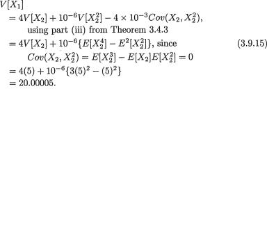
3. Multivariate Random Variables |
151 |
Earlier we had seen applications of this covariance inequality in proving the parts (ii)-(iii) in the Theorem 3.4.2 where we had shown that |ρX1,X2| ≤ 1 whereas |ρX1,X2 | = 1 if and only if X1 = a + bX2 w.p.1.
Example 3.9.5 (Examples 3.2.4, 3.2.5, 3.4.1 Continued) For the two random variables on hand, recall that we had V(X1) = 6.4971 and V(X2) = .6825. Thus, Cov2(X1, X2) ≤ (6.4971)(.6825) ≈ 4.4343. But, we knew that Cov(X1, X2) = –0.2415. !
Example 3.9.6 (Example 3.4.3, 3.4.6 Continued) For the two random variables on hand, recall that we had V(X1) = 3/80 and V(X2) = 19/320. Thus, Cov2(X1, X2) ≤ (3/80)(19/320) = 57/25600 ≈ .00223. But, we had found earlier that Cov(X1, X2) = 3/160 ≈ .01875. !
Example 3.9.7 Suppose that X2 is distributed as N(0, 5) and let X1 = 2X2 – 10–3  Note that V[X2] = 5, but
The covariance inequality (3.9.13) would imply that
However, we know that Cov(X1, X2) = Cov(X2, X1) and hence, by appealing to the Theorem 3.4.3 (ii), we can express Cov(X2, X1) as
The upper bound for Cov2(X1, X2) given by the covariance inequality was 100.00025 whereas the exact value of Cov2(X1, X2) is 100. This upper bound and the actual value of Cov2(X1, X2) are almost indistinguishable because, for all practical purposes, X1 is a linear function of X2. !
152 3. Multivariate Random Variables
3.9.4 Jensen’s and Lyapunov’s Inequalities
Consider a real valued random variable X with finite variance. It is clear that
which would imply that E[X2] ≥ E2[X]. That is, if we let f(x) = x2, then we can claim
The question is this: Can we think of a large class of functions f(.) for which the inequality in (3.9.16) would hold? In order to move in that direction, we start by looking at the rich class of convex functions f(x) of a single real variable x.
Definition 3.9.1 Consider a function f: → . The function f is called convex if and only if
for all u, v and 0 ≤ α ≤ 1. The function f is called concave if and only if
– f is convex.
Figure 3.9.1. A Convex Function f(x)
The situation has been depicted in the Figure 3.9.1. The definition of the convexity of a function demands the following geometric property: Start with any two arbitrary points u, υ on the real line and consider the chord formed by joining the two points (u, f(u)) and (υ, f(υ)). Then, the function f evaluated at any intermediate point z, such as αu + (1 – α)υ with 0 ≤
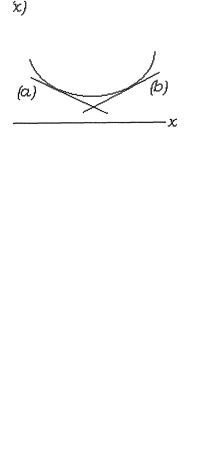
3. Multivariate Random Variables |
153 |
α ≤ 1, will lie under the chord.
Figure 3.9.2. A Convex Function f(x) and Tangent Lines (a), (b)
We may also look at a convex function in a slightly different way. A function f is convex if and only if the curve y = f(x) never goes below the tangent of the curve drawn at the point (z, f(z)), for any z . This has been depicted in the Figure 3.9.2 where we have drawn two tangents labelled as (a) and (b).
In the Figure 3.9.3, we have shown two curves, y = f(x) and y = g(x), x . The function f(x) is convex because it lies above its tangents at any point whatsoever. But, the function g(x) is certainly not convex because a
Figure 3.9.3. Two Functions: f(x) Is Convex, g(x) Is Not Convex
part of the curve y = g(x) lies below the chord as shown which is a violation of the requirement set out in (3.9.17). In the Figure 3.9.3, if we drew the tangent to the curve y = g(x) at the point (u, g(u)), then a part of the curve will certainly lie below this tangent!
Example 3.9.8 Consider the following functions: (i) f(x) = x2 for x ; (ii) f(x) = ex for x ; (iii) f(x) = max(0, x) for x ; and (iv) f(x) = log(x) for x +. The reader should verify geometrically or otherwise that the first three functions are convex, while the fourth one is concave. !
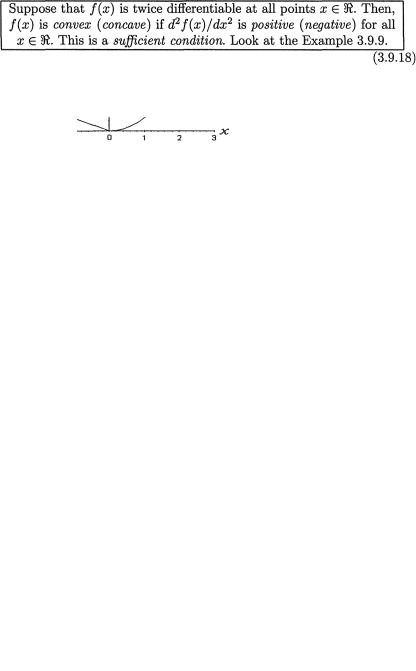
154 3. Multivariate Random Variables
Figure 3.9.4. Plot of f(x) Defined in (3.9.19)
Example 3.9.9 The convexity or concavity of the functions cited in parts (i), (ii) and (iv) of the Example 3.9.8 can be easily checked by verifying the sufficient condition given in (3.9.18). But, a function f(x) may not even be differentiable at all points x , and yet it may be convex (or concave). The function cited in part (iii) of the Example 3.9.8 is of this type. Let us define another function
which has been plotted in the Figure 3.9.4. One should verify that at the point x = 0, the left hand derivative of f(x) is –1 whereas the right hand derivative of f(x) is zero. In other words, the function f(x) is not differentiable at the point x = 0, that is the condition laid out in (3.9.18) is not useful here.
But, after examining the plot of f(x) in the Figure 3.9.4, it becomes apparent that f(x) is indeed a convex function. One should, however, check this claim more formally. !
Theorem 3.9.7 (Jensen’s Inequality) Suppose that X is a real valued random variable and let f(x), x be a convex function. Assume that E[X] is finite. Then, one has
3. Multivariate Random Variables |
155 |
Proof Note that if E[f(X)] is infinite, then the required inequality certainly holds. So, let us assume now that E[f(X)] is finite. Since f(x) is convex, the curve y = f(x) must lie above the tangents at all points (u, f(u)) for any u . With u = E[X], consider specifically the point (u, f(u)) at which the equation of the tangent line would be given by y = f(E[X]) + b{x – E[X]} for some appropriate b. But, then we can claim that
Thus, using (3.9.21), we have
E[f(X)] = E[f(E(X)) + b{X – E(X)}] = f(E(X)) + b{E(X) – E(X)}, which reduces to f(E(X)). Thus, we have the desired result. ¢
In the statement of the Jensen’s inequality (3.9.20), equality holds only when f(x) is linear in x . Also, the inequality in (3.9.20) gets reversed when f(x) is concave.
Example 3.9.10 Suppose that X is distributed as Poisson (λ), λ > 0. Then, using the Jensen’s inequality, for example, we immediately claim that E[X3] > λ3. This result follows because the function f(x) = x3, x + is convex and E[X] = λ. !
Example 3.9.11 Suppose that X is distributed as N(–1, σ2), σ > 0. Then, for example, we have E[|X|] > 1. This result follows immediately from the Jensen’s inequality because the function f(x) = |x|, x is convex and |E[X]| = |–1| = 1. !
Example 3.9.12 Suppose that X is distributed as N(µ, σ2), – ∞ < µ < ∞, σ > 0. Then, for example, we have E[(X – µ)4] ≥ {E[(X – µ)2]}2, by the Jensen’s inequality with f(x) = x2, x + so that one can claim E[(X – µ)4] ≥ (σ2)2 = σ4. !
Example 3.9.13 Suppose that one is proctoring a makeup examination for two students who got started at the same time. Let Xi be the time to complete the examination for the ith student, i = 1, 2. Let X = max (X1, X2), the duration of time the proctor must be present in the room. Then, one has
156 3. Multivariate Random Variables
so that E[X] ≥ max(E[X1], E[X2]). !
Example 3.9.14 Suppose that X is exponentially distributed with mean λ > 0. Then, what can we say about E[X1/2]? Look at the function
for x > 0. This function is concave because f //(x) = –1/4 x–3/2 < 0. Hence, from the Jensen’s inequality we can immediately claim that
Similarly, one can also show that E[log(X)] ≥ log(E[X]) = log(λ). ! What follows is yet another nice application of the Jensen’s inequality.
Theorem 3.9.8 (Lyapunov’s Inequality) Suppose that X is a real valued random variable. Let mr = E1/r[|X|r]. Then, mr is increasing for r ≥ 1.
Proof We want to show that
Observe that
using Jensen’s inequality since f(x) = xr/s, x > 0, is convex. Thus, one has
which is the desired result. ¢
3.9.5 Hölder’s Inequality
In the Cauchy-Schwarz inequality (3.9.10), the upper bound consisted of the product of E[X2] and E[Y2]. However, what if we have a situation like this: For the random variable X, higher than second moments may be assumed finite, but for the random variable Y, lower than second moments may be assumed finite. Under this scenario, the Cauchy-Schwarz inequality does not help much to obtain an upper bound for E2[X1X2]. The following inequality is more flexible. For brevity, we do not supply its proof.
Theorem 3.9.9 (Hölder’s Inequality) Let X and Y be two real valued random variables. Then, with r > 1, s > 1 such that r–1 + s–1 = 1, one has
provided that E[|X|r] and E[|Y|s] are finite.
Example 3.9.15 Suppose that we have two dependent random variables X and Y where X is distributed as N(0, 1), but the pdf of Y is given by

3. Multivariate Random Variables |
157 |
g(y) = 5/3y–8/3 I(1 < y < ∞). Now, by direct integration, one can check that E[Y4/3] is finite but E[Y2] is not. Suppose that we want to get an upper bound for |E[XY]|. The Cauchy-Schwarz inequality does not help because E[Y2] is not finite even though E[X2] is. Let us try and apply the Hölder’s inequality with r = 4 and s = 4/3 in order to obtain
Note that this upper bound is finite whatever be the nature of dependence between these two random variables X and Y. !
3.9.6 Bonferroni Inequality
We had mentioned this inequality in the Exercise 1.3.5, part (ii), for two events only. Here we state it more generally.
Theorem 3.9.10 (Bonferroni Inequality) Consider a sample space S and suppose that ß is the Borel sigma-field of subsets of S. Let A1, ..., Ak be events, that is these belong to ß. Then,
Proof In Chapter 1, we had proved that
so that we can write
This is valid because P(A1 A2) ≤ 1. Similarly, we can write
So, we first verified the desired result for k = 2 and assuming this, we then proved the same result for k = 3. The result then follows by the mathematical induction. ¢
The Exercise 3.9.10 gives a nice application combining the Tchebysheff’s inequality and Bonferroni inequality.

158 3. Multivariate Random Variables
3.9.7 Central Absolute Moment Inequality
Let X be a real valued random variable from some population having its pmf or pdf f(x). Suppose that E[X], that is the population mean, is . In statistics, E[| X – |k] is customarily called the kth central absolute moment of X, k = 1, 2, ... . For example, suppose that X has the following distribution:
X values: |
–1 |
0 |
2 |
2.5 |
Probabilities: |
.1 |
.2 |
.4 |
.3 |
One can check that E[X] = –.1 + 0 + .8 + .75 = 1.45 which is . Now let us fix k = 3 and evaluate the 3rd central absolute moment of X. We have
Now, one may ask: how is the 3rd central absolute moment of X any different from the 3rd central moment of X? One should check that
One thing should be clear. The kth central absolute moment of X should always be non-negative for any k = 1, 2, ... .
Now consider this scenario. Let X1, ..., Xn be real valued random samples from a population having its pmf or pdf f(x). Let the population mean be . One may be tempted to evaluate the average magnitude of the discrepancy
between the sample mean , |
and the population |
mean which will amount to E[| |
– |]. One may even like to evaluate |
E[| – |k] for k = 1, 2, ... . But, then we need the exact distribution of to begin with. From Chapter 4 it will be clear that the determination of the exact distribution of can be hard, even for some of the simplest looking population pmf’s or pdf’s f(x).
The beauty and importance of the next inequality will be appreciated more once we realize that it provides an upper bound for E[|  – |k]
– |k]

3. Multivariate Random Variables |
159 |
even though we may not know the exact distribution of , , k = 1, 2, ... .
The following result actually gives an upper bound for E[| – µ |2ξ] with ξ ≥ 1/2.
Theorem 3.9.11 (Central Absolute Moment Inequality) Suppose that we have iid real valued random variables X1, X2, ... having the common mean µ. Let us also assume that E[| X1 |2ξ] < ∞ for some ξ ≥ 1/2. Then, we have
gwhere k does not depend on n, and T = 2ξ – 1 or ξ according as 1/2 ≤ ξ < 1 or ξ ≥ 1 respectively.
The methods for exact computations of central moments for the sample mean  were systematically developed by Fisher (1928). The classic textbook of Cramér (1946a) pursued analogous techniques extensively. The particular inequality stated here is the special case of a more general large deviation inequality obtained by Grams and Serfling (1973) and Sen and Ghosh (1981) in the case of Hoeffding’s (1948) U-statistics. A sample mean
 turns out to be one of the simplest U-statistics.
3.10Exercises and Complements
3.2.1(Example 3.2.2 Continued) Evaluate f2(i) for i = –1, 0, 1.
3.2.2(Example 3.2.4 Continued) Evaluate E[X1 | X2 = x2] where x2 = 1, 2.
3.2.3(Example 3.2.5 Continued) Check that  = 16.21. Also evaluate
3.2.4Suppose that the random variables X1 and X2 have the following joint distribution.
|
X2 values |
|
X1 values |
|
|
|
|
0 |
1 |
2 |
|
|
|
|
|
|
|
0 |
0 |
3/15 |
3/15 |
|
|
1 |
2/15 |
6/15 |
0 |
|
|
2 |
1/15 |
0 |
0 |
|
|
|
|
|
|
|
|
Using this joint distribution.
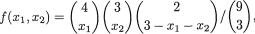
1603. Multivariate Random Variables
(i)find the marginal pmf’s for X1 and X2;
(ii)find the conditional pmf’s f1/2(x1) and f2/1(x2);
(iii)evaluate E[X1 | X2 = x2] and E[X2 | X1 = x1];
(iv)evaluate  and
and 
3.2.5Prove the Theorem 3.2.2.
3.2.6Prove the Theorem 3.2.3.
3.2.7Consider an urn containing sixteen marbles of same size and weight of which two are red, five are yellow, three are green, and six are blue. The marbles are all mixed and then randomly one marble is picked from the urn and its color is recorded. Then this marble is returned to the urn and again all the marbles are mixed, followed by randomly picking a marble from the urn and its color recorded. Again this marble is also returned to the urn and the experiment continues in this fashion. This process of selecting marbles is called sampling with replacement. After the experiment is run n times, sup-
pose that one looks at the number of red (X1), yellow (X2), green (X3) and blue (X4) marbles which are selected.
(i)What is the joint distribution of (X1, X2, X3, X4)?
(ii)What is the mean and variance of X3?
(iii)If n = 10, what is the joint distribution of (X1, X2, X3, X4)?
(iv)If n = 15, what is the conditional distribution of (X1, X2, X3) given that X4 = 5?
(v)If n = 10, calculate P{X1 = 1 ∩ X2 = 3 ∩ X3 = 6 ∩ X4 = 0}.
{Hint: In parts (i) and (v), try to use (3.2.8). In part (ii), can you use (3.2.13)? For part (iii)-(iv), use the Theorem 3.2.2-3.2.3 respectively.}
3.2.8 The mgf of a random vector X = (X1, ..., Xk), denoted by MX(t) with t = (t1, ..., tk), is defined as E[exp{t1X1 + ... + tkXk}]. Suppose that X is distributed as Multk(n, p1, ..., pk). Then,
(i)show that MX(t) = {p1etk}n;
(ii)find the mgf MU(t) of U = X1 + X3 by substituting t1 = t3 = t and ti = 0 for all i ≠ 1, 3 in the part (i). What is the distribution of U?
(iii)use the procedure from part (ii) to find the mgf of the sum of any subset of random variables from X.
3.2.9Suppose that the random variables X1 and X2 have the following joint
pmf:
where x1, x2 are integers, 0 ≤ x1 ≤ 3, 0 ≤ x2 ≤ 3, but 1 ≤ x1 + x2 ≤ 3. Then,
3. Multivariate Random Variables |
161 |
(i)find the marginal pmf’s for X1 and X2;
(ii)find the conditional pmf’s f1/2(x1) and f2/1(x2);
(iii)evaluate E[X1 | X2 = x2] and E[X2 | X1 = x1];
(iv) evaluate E[X |
X ], |
, and |
1 |
2 |
|
3.2.10 Suppose that X = (X1, ..., X5) has the Mult5 (n, p1, ..., p5) with 0 < pi < 1, i = 1, ..., 5, . What is the distribution of Y = (Y1, Y2, Y3) where Y1 = X1 + X2, Y2 = X3, Y3 = X4 + X5? {Hint: Use the Theorem 3.2.2.}
3.2.11 Suppose that X = (X1, X2, X3) has the Mult3 (n, p1, p2, p3) with 0 < pi < 1, i = 1, 2, 3,  Show that the conditional distribution of X1
given that X1 + X2 = r is Bin (r, p1/(p1 + p2)). {Hint: Use the Theorem 3.2.3.} 3.2.12 Suppose that X1 and X2 have the joint pmf
with 0 < p < 1, q = 1 – p. Find the marginal distributions of X1 and X2 and evaluate P{X2 – X1 ≤ 1}.
3.2.13 Suppose that X1 and X2 have the joint pmf
(i)Show that f1(x1) = 1/21 (2x1 + 3) for x1 = 1, 2, 3;
(ii)Show that f2(x2) = 1/7 (x2 + 2) for x2 = 1, 2;
(iii)Evaluate P{X1 ≤ 2} and P{X2 < 2}.
3.2.14 Suppose that X1 and X2 have the joint pdf given by
The surface represented by this pdf is given in the Figure 3.10.1. Show that P{X1 X2 > a} = 1 – a + alog(a) for any 0 < a < 1. {Hint: Note that
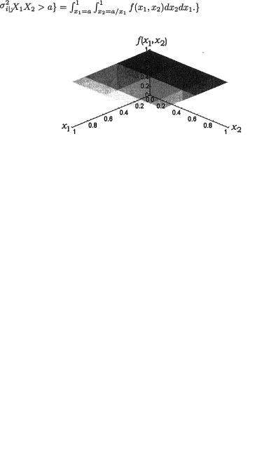
162 3. Multivariate Random Variables
Figure 3.10.1. Plot of the PDF from the Exercise 3.2.14
3.3.1(Examples 3.3.1-3.3.2 Continued) Evaluate E(X1) and V(X1). Also, evaluate 1/2 and 
3.3.2(Examples 3.3.3 Continued) Answer the following questions.
(i)Evaluate E(Xi) and V(Xi), i = 1, 2 using (3.3.19);
(ii)Evaluate E[X1(1 – X1)],  and E[(X1 + X2)2];
(iii)Show that fi|j(xi) = fi(xi) for i ≠ j = 1, 2.
3.3.3(Example 3.3.5 Continued) Evaluate E(Xi) and V(Xi), i = 1, 2. Evaluate i|j and  for i ≠ j, i, j = 1, 2. Also evaluate
3.3.4Let c be a positive constant such that X1 and X2 have the joint pdf
given by
Find the value of c. Derive the expressions of f1 |
(x1), f2(x |
2), f1/2(x1), and |
|
f2/1(x2). Evalute E(Xi) and V(Xi), i = 1, 2. Evaluate i|j and |
for i ≠ j, |
||
i, j = 1, 2. Also evaluate E[X1 (1 – X1)], |
|
|
and E[(X1 + |

3. Multivariate Random Variables |
163 |
X2)2]. The surface represented by this pdf is given in the Figure 3.10.2.
Figure 3.10.2. Plot of the PDF from the Exercise 3.3.4 with c = 3/16
3.3.5 Let c be a positive constant such that X1 and X2 have the joint pdf given by
Find the value of c. Derive the expressions of f1(x1), f2(x2), f1/2(x1), and f2/1(x2). Does either of X1, X2 have a standard distribution which matches with one of
those distributions listed in Section 1.7? Evaluate E(Xi) and V(Xi), i = 1, 2. Evaluate i/j and  for i ≠ j, i, j = 1, 2. Also evaluate E[X1(1 – X1)],
  and E[(X1 + X2)2]. The surface represented by this pdf is
given in the Figure 3.10.3.
Figure 3.10.3. Plot of the PDF from the Exercise 3.3.5 with c = 1
3.3.6 (Example 3.3.10 Continued) Evaluate E[X1 X2] and E[X1  Also evaluate E[X1(1 – X1)], E[X1 X2
  ] and E[X1 + X2 + X3)2].
3.3.7 (Example 3.3.10 Continued) Find the expressions for E[X1 | X2 = x2, X3 = x3] and E[X1  | X2 = x2] with 0 < x2 < 2, 0 < x3 < 1.
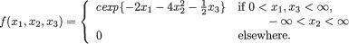
164 3. Multivariate Random Variables
{Hints: First find the conditional pdf’s of X1 given X2 = x2, X3 = x3 and that of (X1, X3) given X2 = x2. Next, express the expected values as the respective integrals and then evaluate them.}
3.3.8 (Example 3.3.10 Continued) Choose any three specific pdf’s on three finite intervals as ai(xi), i = 1, 2, 3. Then, construct an appropriate combination of these ai’s to define a pdf f(x) along the line of (3.3.47). Try putting these components in a certain order and adjust the coefficients so that the whole integral is one. {Hint: Examine closely why we had the success in the equation (3.3.48).}
3.3.9 (Example 3.3.11 Continued) Evaluate E[X1 X2 X5] and E[ X5].
X5].
Also evaluate E[X1(1 – X5)], E[X1 X2(2 – X3)2] and E[(X1 + X2 + X3 + X4 + X5)2].
3.3.10 (Example 3.3.11 Continued) Find the expressions for E[X1(1 – X5)
| X2 = x2, X4 = x4] and E[X1  | X5 = x5] with 0 < x2 < 2, 0 < x4, x5 < 1. {Hints: First find the conditional pdf’s of (X1, X5) given X2 = x2, X4 = x4 and that of
(X1, X3) given X5 = x5. Next, express the expected values as the respective integrals and then evaluate them.}
3.3.11(Example 3.3.11 Continued) Choose any five specific pdf’s on five
finite intervals as ai(xi), i = 1, ..., 5. Then, construct an appropriate combination of these ai’s to define a pdf f(x) along the line of (3.3.53). Try putting these components in a certain order and adjust the coefficients so that the whole integral is one. {Hint: Examine closely how we had defined the function f in the equation (3.3.53).}
3.3.12Let c be a positive constant such that X1, X2 and X3 have the joint pdf given by
Find the value of c. Derive the marginal pdf’s of X1, X2 and X3. Does either of X1, X2, X3 have a standard distribution which matches with one of those distributions listed in Section 1.7? Evaluate E[X1 X2] and E[X1  ]. Also evaluate E[X1(1 – X1)], E[X1 X2
  ] and E[(X1 + X2 + X3)2].
3.4.1(Example 3.2.1 Continued) In the case of the random variables X1, X2 whose joint pdf was defined in the Table 3.2.1, calculate ρ, the correlation coefficient between X1 and X2.
3.4.2(Exercise 3.2.4 Continued) In the case of the random variables X1, X2 whose joint pdf was defined in the Exercise 3.2.4, calculate ñ, the correlation coefficient between X1 and X2.

3. Multivariate Random Variables |
165 |
3.4.3 (Example 3.3.10 Continued) Evaluate Cov(Xi, Xj), i ≠ j = 1, 2, 3. Then, evaluate ρXi, Xj, i ≠ j = 1, 2, 3.
3.4.4 (Example 3.3.11 Continued) Evaluate Cov(Xi, Xj), i ≠ j = 1, ..., 5. Then, evaluate ρXi, Xj, i ≠ j = 1, ..., 5.
3.4.5Prove the Theorem 3.4.3.
3.4.6With any two random variables X1 and X2, show that
provided that Cov(X1, X2), V(X1), and V(X2) are finite.
3.4.7 (Exercise 3.4.6 Continued) Consider any two random variables X1 and X2 for which one has V(X1) = V(X2). Then, for this pair of random variables X1 and X2 we must have Cov(X1, X2) = 0. Next, using this ammunition, construct several pairs of random variables which are uncorrelated.
3.4.8 (Examples 3.2.6-3.2.7 Continued) Consider the multinomial random variable X = (X1, ..., X6) defined in the Example 3.2.6. Evaluate ρXi, Xj for all i ≠ j = 1, ..., 6.
3.4.9 (Example 3.2.8 Continued) Consider the multinomial random variable X = (X1, X5,  ) defined in the Example 3.2.6 with
  = n – (X1 + X5). Evaluate ρX1, X5, ρX1,
 and ρX5,
 .
.
3.4.10 (Exercise 3.2.7 Continued) Consider the multinomial random variable X = (X1, X2, X3, X4) defined in the Exercise 3.2.7. Evaluate ρXi, Xj for all i ≠ j = 1, 2, 3, 4.
3.4.11 (Exercise 3.2.10 Continued) Recall that X = (X1, ..., X5) has the
Mult5(n, p1, ..., p5) with 0 < pi < 1, i = 1, ..., 5, whereas Y = (Y1, Y1,2,2,Y33.) where Y1 = X1 + X2, Y2 = X3, Y3 = X4 + X5. Evaluate ρYi, Yj for all i ≠ j =
3.4.12 Suppose that X1 and X2 have the joint pdf given by
(i)Show that f1(x1) = x1 + 1/2, f2(x2) = x2 + 1/2 for 0 < x1, x2 < 1;
(ii)Evaluate P{1/2 ≤ X1 ≤ 3/4 | 1/3 ≤ X2 ≤ 2/3}.
3.4.13Suppose that X1 and X2 have the joint pdf given by
166 3. Multivariate Random Variables
Show that ρX1, X2 = – 5/139.
3.5.1 (Exercise 3.3.4 Continued) Let c be a positive constant such that X1 and X2 have the joint pdf given by
Prove whether or not X1 and X2 are independent. Solve this exercise first by directly applying the Definition 3.5.1. Then, repeat this exercise by applying the Theorem 3.5.3.
3.5.2 (Exercise 3.3.5 Continued) Let c be a positive constant such that X1 and X2 have the joint pdf given by
Prove whether or not X1 and X2 are independent. Solve this exercise first by directly applying the Definition 3.5.1. Then, repeat this exercise by applying the Theorem 3.5.3.
3.5.3 (Exercise 3.3.12 Continued) Let c be a positive constant such that X1, X2 and X3 have the joint pdf given by
Prove whether or not X1, X2 and X3 are independent. Solve this exercise first by directly applying the Definition 3.5.1. Then, repeat this exercise by applying the Theorem 3.5.3.
3.5.4(Example 3.5.4 Continued) Verify all the steps in the Example 3.5.4.
3.5.5(Example 3.5.4 Continued) In the Example 3.5.4, suppose that we fix f1(x1) = 2x1,  and ,
and ,  0 < x1, x2, x3 < 1.
Then, form the function g(x1, x2, x3) as in (3.5.2).
(i)Directly by integration, check, that g(x1, x2, x3) is a pdf;
(ii)Directly by integration, find the expressions of all pairwise marginal pdf’s gi,j(xi, xj) and single marginal pdf’s gi(xi) for i ≠ j = 1, 2, 3;
(iii)Show directly that the X’s are pairwise independent, but X1, X2, X3 are not independent.
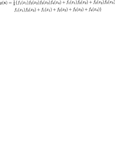
3. Multivariate Random Variables |
167 |
3.5.6(Example 3.5.4 Continued) Construct some other specific functions
fi(xi), i = 1, 2, 3 satisfying the conditions laid out in the Example 3.5.4 and observe what happens in some of those special situations.
3.5.7Let us start with the non-negative integrable functions fi(xi) for 0 < x
<1 which are not identically equal to unity such that we can claim:  fi(xi)dxi = 1, i = 1, 2, 3, 4. With x = (x1, x2, x3, x4), let us then define
for 0 < xi < 1, i = 1, 2, 3, 4.
(i)Directly by integration, check that g(x1, x2, x3, x4) is a pdf;
(ii)Directly by integration, find the expression of the marginal pdf
g1, 2,3(x1, x2, x3);
(iii)Show directly that X1, X2, X3 are independent;
(iv)Consider the random variables X1, X2, X3, X4 whose joint pdf is given by g(x1, x2, x3, x4). Show that X1, X2, X3, X4 are not indepen dent.
3.5.8(Exercise 3.5.7 Continued) Along the lines of the Exercise 3.5.6,
construct some specific functions fi(xi), i = 1, 2, 3, 4 satisfying the conditions laid out in the Exercise 3.5.7 and observe what happens in some of those special situations.
3.5.9Prove the Theorem 3.5.3.
3.5.10Suppose that X1 and X2 have the joint pmf
Prove whether or not X1 and X2 are independent. 3.5.11 Suppose that X1 and X2 have the joint pmf
Prove that X1 and X2 are dependent.
3.5.12 Suppose that X1 and X2 have the joint pmf
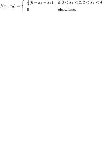
168 3. Multivariate Random Variables
Prove whether or not X1 and X2 are independent.
3.5.13 Suppose that X1 and X2 have the joint pmf such that P{X1 = 2 ∩ X2
= 3} = 1/3, P{X1 = 2 ∩ X2 = –1} = a, P{X1 = –1 ∩ X2 = 3} = b and P{X1 = –1 ∩ X2 = –1} = 1/6 where a and b are appropriate numbers. Determine a and
b when X1 and X2 are independent.
3.5.14 Suppose that X1 and X2 have the joint pdf
where k is a positive constant.
(i)Show that k = 2;
(ii)Show that f1(x1) = 2{e–x1 – e–2x1} I(0 < x1 < ∞) and f2(x2) = 2e–2x2 I(0 < x2 < ∞). Find P(X2 ≥ 3);
(iii)Show that f1/2(x1) = e–(x1 – x2) I(x2 < x1 < ∞) and f2/1(x2) = e–x2 (1 –e–x1)–1 I(0 < x2 < x1);
(iv)Prove whether or not X1 and X2 are independent.
3.5.15Suppose that X1 and X2 have the joint pdf
(i)Show that f1(x1) = ¼(3 – x1) I(0 < x1 < 2) and f2(x2) = ¼(5 – x2) I(2 <x2 < 4);
(ii)Show that f1/2(x1) =  I(0 < x1 < 2, 2 < x2 < 4) and f2/1(x2) =
  I(0 < x1 < 2, 2 < x2 < 4);
(iii)Prove whether or not X1 and X2 are independent.
3.5.16 Suppose that X1 and X2 have the joint pdf
The surface represented by this pdf is given in the Figure 3.10.4.
3. Multivariate Random Variables |
169 |
(i)Show that f1(x1) = ¼π{cos(½πx1) + sin(½πx1)} for 0 < x1 < 1, and f2(x2) = ¼π{cos(½πx2) + sin(½πx2)} for 0 < x2 < 1;
(ii)Prove whether or not X1 and X2 are independent.
Figure 3.10.4. Plot of the PDF from the Exercise 3.5.16
3.5.17 Suppose that the random vector X = (X1, X2, X3, X4) has its joint pdf given by
(i)Find the marginal pdf’s fi(xi), i = 1, 2, 3, 4. Show that each Xi is distributed as N(0, 4), i = 1, 2, 3, but X4 is distributed as N(0, 1);
(ii)By integrating f(x1, x2, x3, x4) with respect to x4 alone, obtain the joint pdf of (X1, X2, X3);
(iii)Combine the parts (i) and (ii) to verify that X1, X2, X3 form a set of independent random variables;
(iv)Show that X1, X2, X3, X4 do not form a set of independent random variables.
3.5.18(Exercise 3.5.17 Continued) Consider the random vector X = (X1, X2, X3, X4) with its joint pdf given in the Exercise 3.5.17. Using this random vector X, find few other four-dimensional random vectors Y = (Y1, Y2, Y3, Y4) where Y1, Y2, Y3 are independent, but Y1, Y2, Y3, Y4 are not.
3.5.19Suppose that X has the following pdf with –∞ < µ < ∞, 0 < σ < ∞:
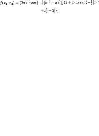
170 3. Multivariate Random Variables
One will recall from (1.7.27) that this pdf is known as the lognormal density and the corresponding X is called a lognormal random variable. Suppose that X1, X2 are iid having the common pdf f(x). Let r and s be arbitrary, but fixed real numbers. Then, obtain the expression for 
3.6.1Derive the marginal pdf of X1 in the Theorem 3.6.1, part (i).
3.6.2Prove Theorem 3.6.1, part (iii).
3.6.3(Example 3.6.2 Continued) Suppose that (X1, X2) is distributed as N2(0, 0, 1, 1, ρ) where one has ρ (–1, 1). Find the expression of the mgf of the random variable X1 X2, that is E{exp[tX1 X2]} for t belonging to an appropriate subinterval of .
3.6.4Suppose that the joint pdf of (X1, X2) is given by
for –∞ < x1, x2 < ∞. Evaluate E[Xi], V[Xi] for i = 1, 2, and ρX1, X2. 3.6.5 Suppose that the joint pdf of (X1, X2) is given by
for –∞ < x1, x2 < ∞ where k is a positive number. Evaluate E[Xi], V[Xi]
for i = 1, 2, and ρX1, X2.
3.6.6 Suppose that (X1, X2) is distributed as N2(3, 1, 16, 25, 3/5). Evaluate P{3 < X2 < 8 | X1 = 7} and P{–3 < X1 < 3 | X2 = –4}.
3.6.7 Suppose that X1 is distributed as N(µ, σ2) and conditionally the distribution of X2 given that X1 = x1 is N(x1, σ2). Then, show that the joint distribution of (X1, X2) is given by N2(µ, µ, σ2, 2σ2,  ).
).
3.6.8 Suppose that the joint pdf of (X1, X2) is given by
for –∞ < x1, x2 < ∞.
(i)By direct integration, verify that f(x1, x2) is a genuine pdf;
(ii)Show that the marginal distributions of X1, X2 are both univariate normal;
(iii)Does this f(x1, x2) match with the density given by (3.6.1)? 3.6.9 Suppose that the joint pdf of (X1, X2, X3) is given by

3. Multivariate Random Variables |
171 |
for –∞ < x1, x2, x3 < ∞. Show that X1, X2, X3 are dependent random variables. Also show that each pair (X1, X2), (X2, X3) and (X1, X3) is distributed as a bivariate normal random vector.
3.7.1 This exercise provides a discrete version of the Example 3.7.1. Suppose that a random variable X1 has the following probability distribution.
|
X1 values: |
|
–5 |
–2 |
0 |
2 |
5 |
|
Probabilities: |
.25 |
.2 |
.1 |
.2 |
.25 |
|
Define |
Then, show that |
|
|
|
|
||
(i) |
E[X1] = |
] = 0; |
|
|
|
|
|
(ii)Cov(X1, X2) = 0, that is the random variables X1 and X2 are uncorrelated;
(iii)X1 and X2 are dependent random variables.
3.7.2(Exercise 3.7.1 Continued) From the Exercise 3.7.1, it becomes clear that a statement such as “the zero correlation need not imply independence” holds not merely for the specific situations handled in the Examples 3.7.1-3.7.2. Find a few other examples of the type considered in the Exercise 3.7.1.
3.7.3In view of the Exercises 3.7.1-3.7.2, consider the following gener-
alization. Suppose that X1 has an arbitrary discrete distribution, symmetric about zero and having its third moment finite. Define .  Then, show that
(i)E[X1] = E[  ] = 0;
(ii)Cov(X1, X2) = 0, that is the random variables X1 and X2 are uncorrelated;
(iii)X1 and X2 are dependent random variables.
3.7.4(Example 3.7.1 Continued) In the Example 3.7.1, we used nice tricks with the standard normal random variable. Is it possible to think of another example by manipulating some other continuous random variable to begin
with? What if one starts with X1 that has a continuous symmetric distribution about zero? For example, suppose that X1 is distributed uniformly on the interval (–1, 1) and let  Are X1 and X2 uncorrelated, but dependent? Modify this situation to find other examples, perhaps with yet some other continuous random variable X1 defined on the whole real line and
3.7.5In the types of examples found in the Exercises 3.7.1-3.7.4, what if
someone had defined  instead? Would X1 and X2 thus defined, for example, be uncorrelated, but dependent in the earlier exercises?
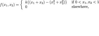
1723. Multivariate Random Variables
3.7.6(Example 3.7.3 Continued) The zero correlation between two random variables sometimes does indicate independence without bivariate normality. The Example 3.7.3 had dealt with a situation like this. In that example,
will the same conclusion hold if both X1 and X2 were allowed to take two arbitrary values other than 0 and 1? {Hint: First recall from the Theorem
3.4.2, part (i) that the correlation coefficient between X1 and X2 would be the same as that between Y1 and Y2 where we let Yi = (Xi – aibi, with ai , bi+ being any fixed numbers. Then, use this result to reduce the given problem to a situation similar to the one in the Example 3.7.3.}
3.7.7Suppose that X1 and X2 have the joint pdf
where k is some positive constant. Show that X1 and X2 are uncorrelated, but these are dependent random variables.
3.7.8 Suppose that X1 and X2 have the joint pdf
for –∞ < x1, x2 < ∞. Show that X1 and X2 are uncorrelated, but these are dependent random variables.
3.7.9 (Example 3.7.4 Continued) Suppose that (U1, U2) is distributed as
N2(5, 15, 8, 8, ρ) for some ρ (–1, 1). Let X1 = U1 + U2 and X2 = U1 – U2. Show that X1 and X2 are uncorrelated.
3.8.1Verify the entries given in the Table 3.8.1.
3.8.2Consider the Beta(α, β) distribution defined by (1.7.35). Does the pdf belong to the appropriate (that is, one-or two-parameter) exponential family when
(i)α is known, but β is unknown?
(ii)β is known, but α is unknown?
(iii)α and β are both unknown?
3.8.3 Consider the Beta(α, β) distribution defined by (1.7.35). Does the pdf belong to the appropriate (that is, oneor two-parameter) exponential family when
(i)α = β = θ, but θ(> 0) is unknown?
(ii)α = θ, β = 2θ, but θ(> 0) is unknown?
3.8.4 Suppose that X has the uniform distribution on the interval (–θ, θ) with θ(> 0) unknown. Show that the corresponding pdf does not belong to
3. Multivariate Random Variables |
173 |
the one-parameter exponential family defined by (3.8.1). {Hint: Use ideas similar to those from the Example 3.8.5.}
3.8.5 Consider two random variables X1, X2 whose joint pdf is given by
with θ(> 0) unknown.
(i)Are X1, X2 independent?
(ii)Does this pdf belong to the one-parameter exponential family?
3.8.6Does the multinomial pmf with unknown parameters p1, ..., pk defined in (3.2.8) belong to the multi-parameter exponential family? Is the number of parameters k or k – 1?
3.8.7Express the bivariate normal pdf defined in (3.6.1) in the form of an appropriate member of the one-parameter or multi-parameter exponential family in the following situations when the pdf involves
(i)all the parameters µ1, µ2, σ1, σ2, ρ;
(ii)µ1 = µ2 = 0, and the parameters σ1, σ2, ρ;
(iii)σ1 = σ2 = 1, and the parameters µ1, µ2, ρ;
(iv)σ1 = σ2 = σ, and the parameters µ1, µ2, σ, ρ;
(v)µ1 = µ2 = 0, σ1 = σ2 = 1, and the parameter ρ.
3.8.8 Consider the Laplace or the double exponential pdf defined as
for –∞ < x, θ < ∞ where θ is referred to as a parameter. Show that f(x; θ) does not belong to the one-parameter exponential family.
3.8.9 Suppose that a random variable X has the Rayleigh distribution with
where θ(> 0) is referred to as a parameter. Show that f(x; θ) belongs to the one-parameter exponential family.
3.8.10 Suppose that a random variable X has the Weibull distribution with
where α(> 0) is referred to as a parameter, while β(> 0) is assumed known. Show that f(x; α) belongs to the one-parameter exponential family.
3.9.1(Example 3.9.4 Continued) Prove the claim made in the Example
3.9.4which stated the following: Suppose that X is a random variable whose mgf MX(t) is finite for some t Τ (–∞, 0). Then, it follows
174 3. Multivariate Random Variables
from the Theorem 3.9.2 that for any fixed real number a, one has P{X ≤
3.9.2 Suppose that X has the Gamma(4, 1/2) distribution.
(i) Use Markov inequality to get an upper bound for P{X ≥ 12};
(ii) Use Bernstein-Chernoff inequality to get an upper bound for P{X ≥ 12};
(iii) Use Tchebysheff’s inequality to obtain an upper bound for P{X ≥ 12}.
3.9.3 (Exercise 3.6.6 Continued) Suppose that (X1, X2) is distributed as N2(3, 1, 16, 25, 3/5).
(i)Use Tchebysheff’s inequality to get a lower bound for P{–2 < X2 < 10 | X1 = 7};
(ii)Use Cauchy-Schwarz inequality to obtain an upper bound for (a) E[|X1X2|] and (b) 
{Hint: In part (i), work with the conditional distribution of X2 | X1 = 7 and from X2, subtract the right conditional mean so that the Tchebysheff’s inequality can be applied. In part (ii), apply the Cauchy-Schwarz inequality in a straightforward manner.}
3.9.4Suppose that X is a positive integer valued random variable and
denote pk = P(X = k), k = 1, 2, ... . Assume that the sequence {pk; k ≥ 1} is non-increasing. Show that pk ≥ 2k–2 E[X] for any k = 1, 2, ... . {Hint: E[X] ≥  Refer to (1.6.11).}
3.9.5Suppose that X is a discrete random variable such that P(X = –a) =
P(X = a) = 1/8 and P(X = 0) = 3/4 where a(> 0) is some fixed number. Evaluate µ, σ and P(|X| ≥ 2σ). Also, obtain Tchebysheff’s upper bound for P(|X| ≥ 2σ). Give comments.
3.9.6Verify the convexity or concavity property of the following func-
tions.
(i)h(x) = x5 for –1 < x < 0;
(ii)h(x) = |x|3 for x ;
(iii)h(x) = x4e–2x for x +;
(iv)h(x) = e–1/2x2 for x ;
(v)h(x) = x–1 for x +.
3.9.7 Suppose that 0 < α, β < 1 are two arbitrary numbers. Show that
{Hint: Is log(x) with x > 0 convex or concave?}
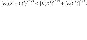
3. Multivariate Random Variables |
175 |
3.9.8 First show that f(x) = x–1 for x + is a convex function. Next, suppose that X is a real valued random variable such that P(X > 0) = 1 and E[X] is finite. Show that
(i)E[1/X] > 1/E[X];
(ii)Cov(X, 1/X) < 0.
3.9.9 Suppose that X and Y are two random variables with finite second moments. Also, assume that P(X + Y = 0) < 1. Show that
{Hint: Observe that (X + Y)2 ≥ |X|{|X + Y|} + |Y|{|X + Y|}. Take expectations throughout and then apply the Cauchy-Schwarz inequality on the rhs.}
3.9.10 Suppose that X1, ..., Xn are arbitrary random variables, each with zero mean and unit standard deviation. For arbitrary ε(> 1), show that
{Hint: Let Ai be the event that  , i = 1, ..., n. By Tchebysheff’s inequality, P(Ai) ≥ 1 – (nε2)–1, i = 1, ..., n. Then apply Bonferroni inequality, namely,
  ≥ n{1 – (nε2)–1} – (n–1) = 1 – ε–2.}
3.9.11Suppose that Y is a random variable for which E[Y] = 3 and E[Y2]
=13. Show that P{–2 < Y < 8} > 21/25. {Hint: Check that V[Y] = 4 so that P{–2 < Y < 8} = P{|Y – 3| < 5} > 1 – 4/25 = 21/25, by Tchebysheff’s inequality.}
This page intentionally left blank
4
Functions of Random Variables
and Sampling Distribution
4.1 Introduction
It is often the case when we need to determine the distribution of a function of one or more random variables. There is, however, no one unique approach to achieve this goal. In a particular situation, one or more approaches given in this chapter may be applicable. Which method one would ultimately adopt in a particular situation may largely depend on one’s taste. For completeness, we include standard approaches to handle various types of problems involving transformations and sampling distributions.
In Section 4.2 we start with a technique involving distribution functions. This approach works well in the case of discrete as well as continuous random variables. Section 4.2 also includes distributions of order statistics in the continuous case. Next, Section 4.3 demonstrates the usefulness of a moment generating function (mgf) in deriving distributions. Again, this approach is shown to work well in the case of discrete as well as continuous random variables. Section 4.4 exclusively considers continuous distributions and transformations involving one, two, and several random variables. One highlight in this section consists of the Helmert (Orthogonal) Transformation in the case of a normal distribution, and another consists of a transformation involving the spacings between the successive order statistics in the case of an exponential distribution. In both these situations, we deal with one-to-one transformations from n random variables to another set of n random variables, followed by discussions on Chi-square, Student’s t, and F distributions. Section 4.5 includes sampling distributions for both one-sample and two-sample problems. Section 4.6 briefly touches upon the multivariate normal distributions and provides the distribution of the Pearson correlation coefficient in the bivariate normal case. Section 4.7 shows, by means of several examples, the importance of independence of various random variables involved in deriving sampling distributions such as the Student’s t and F distributions as well as in the reproductive properties of normal and Chi-square random variables.
The following example shows the immediate usefulness of results which evolve via transformations and sampling distributions. We first solve the
177
178 4. Functions of Random Variables and Sampling Distribution
problem using the direct calculation, and then provide an alternative quick and painless way to solve the same problem by applying a result derived later in this chapter.
Example 4.1.1 Let us consider a popular game of “hitting the bull’s eye” at the point of intersection of the horizontal and vertical axes. From a fixed distance, one aims a dart at the center and with the motion of the wrist, lets it land on the game board, say at the point with the rectangular coordinates (Z1, Z2). Naturally then, the distance (from the origin) of the point on the game board where the dart lands is A smaller distance would indicate better performance of the player. Suppose that Z1 and Z2 are two independent random variables both distributed as N(0, 1). We wish to calculate
 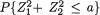 where a > 0, that is the probability that the thrown dart lands within a distance of
  from the aimed target. The joint pdf of (Z1, Z2) would obviously amount to
  )} with
–∞ < z1, z2 < ∞. We then go back to the heart of (3.3.20) as we proceed to evaluate the double integral,
Let us substitute
which transform a point (z1, z2) on the plane in the rectangular coordinates system to the point (r, θ) on the same plane, but in the polar coordinates system. Now, the matrix of the first partial derivatives of z1 and z2 with respect to θ and r would be
so that its determinant, det(A) = ½. Now, we can rewrite the double integral from (4.1.1) as
But, later in this chapter (Example 4.3.6), we show that the distribution of  is indeed
  , that is a Chi-square with two degrees of

4. Functions of Random Variables and Sampling Distribution |
179 |
freedom. Thus the pdf of W is given by g(w) = 1/2exp{–1/2ω}I(ω > 0). Refer to Section 1.7 as needed. The required probability, P(W ≤ a) is simply then
which matches with the answer found earlier in (4.1.3). This second approach appears much simpler. !
In the Exercise 4.1.1, we have proposed a direct approach to evaluate ,with some fixed but arbitrary b > 0, where Z1, Z2 are iid standard normal. The Exercise 4.5.4, however, provides an easier way to evaluate
the same probability by considering the sampling distribution of the random variable Z1/Z2 which just happens (Exercise 4.5.1 (iii)) to have the Cauchy distribution defined in (1.7.31). The three Exercises 4.5.7-4.5.9 also fall in the same category.
4.2 Using Distribution Functions
Suppose that we have independent random variables X1, ..., Xn and let us denote Y = g (X1, ..., Xn), a real valued function of these random variables. Our goal is to derive the distribution of Y.
If X1, ..., Xn or Y happen to be discrete random variables, we set out to evaluate the expression of P(Y = y) for all appropriate y y, and then by identifying the form of P(Y = y), we are often led to one of the standard distributions.
In the continuous case, the present method consists of first obtaining the distribution function of the new random variable Y, denoted by F(y) = P(Y ≤ y) for all appropriate values of y y. If F(y) is a differentiable function of Y, then by differentiating F(y) with respect to y, one can obtain the pdf of Y at the point y. In what follows, we discuss the discrete and continuous cases separately.
4.2.1 Discrete Cases
Here we show how some discrete situations can be handled. The exact techniques used may vary from one problem to another.
Example 4.2.1 Suppose that X1, X2 are two independent random variables having respectively the following probability distributions:
X1 values: |
0 |
1 |
3 |
Probabilities: |
.2 |
.3 |
.5 |
|
|
|
|
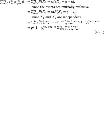
180 4. Functions of Random Variables and Sampling Distribution
X2 values: |
–1 |
0 |
2 |
2.5 |
Probabilities: |
.1 |
.2 |
.4 |
.3 |
Now, P(X1 = x1 ∩ X2 = x2) = P(X1= x1)P(X2 = x2) for all X1 = 0, 1, 3 and X2 = –1, 0, 2, 2. 5. Suppose that we want to obtain the pmf for the random variable
Y = X1 + X2. The possible values Y of Y belong to the set γ = {–1, 0, 1, 2, 2.5,
3, 3.5, 5, 5.5}. Now P(Y = 0) = P(X1 = 0 ∩ X2 = 0) + P(X1 = 1 ∩ X2 = –1) = 1 ∩ X2 = –1) = (.2)(.2) + (.3)(.1) = .07. Also, P(Y = 2) = P(X1 = 0 ∩ X2 = 2)
+ P(X1 = 3 ∩ X2 = –1) = (.2)(.4) + (.5)(.1) = .13, and this way the pmf function g(y) = P(Y = y) can be obtained for all y y. "
Example 4.2.2 Let X1 and X2 be independent random variables, where X1 is Binomial(n1, p) and X2 is Binomial(n2, p) with 0 < p < 1. Let us find the distribution of Y = X1 + X2. With 0 ≤ Y ≤ n1 + n2, one can express P(Y = Y) as
In order to evaluate the summation in the last step in (4.2.1), one needs to compare the coefficients of py(1 – p)n1+n2–y on both sides of the identity:
Hence, can be replaced bY , a fact that follows from the Binomial Theorem (see (1.4.12)). That is, we can simply rewrite
which is the pmf of the Binomial(n1 + n2, p) variable. Hence, the random variable Y has the Binomial (n1 + n2 p) distribution. !
Example 4.2.3 Suppose that X1, ..., Xk are independent, Xi is distributed as
the Binomial(ni, p), 0 < p < 1, i = 1, ..., k. Obviously X1 + X2 + X3 = {X1 + X2} + X3, and of course X1 + X2 and X3 are independently distributed as
the binomials with the same p. Hence, using the Example 4.2.2, we conclude that X1 + X2 + X3 is Binomial({n1 + n2} + n3, p), because we are simply adding two independent Binomial random variables

4. Functions of Random Variables and Sampling Distribution |
181 |
respectively with parameters (n1 + n2, p) and (n3, p). Next, one may use mathematical induction to claim that is thus distributed as the Binomial ( ). !
). !
4.2.2 Continuous Cases
The distribution function approach works well in the case of continuous random variables. Suppose that X is a continuous real valued random variable and let Y be a real valued function of X. The basic idea is first to express the distribution function G(y) = P(Y ≤ y) of Y in the form of the probability of an appropriate event defined through the original random variable X. Once the expression of G(y) is found in a closed form, one would obviously obtain dG(y)/dy, whenever G(y) is differentiable, as the pdf of the transformed random variable Y in the appropriate domain space for y. This technique is ex- plained with examples.
Example 4.2.4 Suppose that a random variable X has the pdf
Let Y = X2 and we first obtain G(y) = P(Y ≤ y) for all y in the real line. Naturally, G(y) = 0 if y ≤ 1 and G(y) = 1 if y ≥ 4. But, for 1 < y < 4, we have  . Hence,
which is the pdf of Y. !
In a continuous case, for the transformed variable Y = g(X), first find the df G(y) = P(Y ≤ y) of Y in the appropriate space for Y. Then, G(y), whenever G(y) is differentiable, would be pdf of Y for the appropriate y values.
Example 4.2.5 Let X have an arbitrarY continuous distribution with its pdf f(x) and the df F(x) on the interval (a, b) . We first find the pdf of the random variable F(X) and denote W = F(X). Let F–1(.) be the inverse function of F(.), and then one has for 0 < w < 1:
and thus the pdf of W is given by

182 4. Functions of Random Variables and Sampling Distribution
That is, W has a uniform distribution on the interval (0, 1). Next, define U = – log (F(X)) and V = –2log(F(X)). The domain space of U and V are both (0, ∞). Now, for 0 < u < ∞, one has the df of U,
so that U has the pdf f(u) =  G(u) = e–u, which corresponds to the pdf of a
standard exponential random variable which is defined as Gamma(1, 1). Refer to (1.7.24). Similarly, for 0 < v < ∞, we write the df of V,
so that V has the pdf g(v) =  H(v) = ½e–1/2v, which matches with the pdf of
a Chi-square random variable with two degrees of freedom. Again refer back to Section 1.7 as needed. !
Example 4.2.6 Suppose that Z has a standard normal distribution and let Y = Z2. Denote (.) and Φ (.) respectively for the pdf and df of Z. Then, for 0 < y < ∞, we have the df of Y,
and hence the pdf of Y will be given by
Now g(y) matches with the pdf of a Chi-square random variable with one degree of freedom. That is, Z2 is distributed as a Chi-square with one degree of freedom. Again, refer back to Section 1.7. !
Suppose that X has a continuous random variable with its df F(x). Then, F(X) is Uniform on the interval (0, 1), –log{F(X)} is standard exponential, and –2log{F(X)} is 
4.2.3 The Order Statistics
Let us next turn to the distributions of order-statistics. Consider independent and identically distributed (iid) continuous random variables X1, ..., Xn having
the common pdf f(x) and the df F(x). Suppose that Xn:1 ≤ Xn:2 ≤ ... ≤ Xn:n stand for the corresponding ordered random variables where Xn:i is referred to as
the ith order statistic. Let us denote Yi = Xn:i for i = 1, ..., n and Y = (y1, ..., yn). The joint pdf of Y1, ..., Yn, denoted by fY(y1, ..., yn), is given by

4. Functions of Random Variables and Sampling Distribution |
183 |
In (4.2.2), the multiplier n! arises because y1, ..., yn can be arranged among themselves in n! ways and the pdf for any such single arrangement amounts to  . Often we are specifically interested in the smallest and largest order statistics. For the largest order statistic Yn, one can find the distribution as follows:
and hence the pdf of Yn would be given by
in the appropriate space for the Y values. In the same fashion, for the smallest order statistic Y1, we can write:
and thus the pdf of Y1 would be given by
in the appropriate space for the Y values.
In the Exercise 4.2.5, we have indicated how one can find the joint pdf of anY two order statistics Yi = Xn:i and Yj = Xn:j.
Using the Exercise 4.2.5, one can derive the joint pdf of Y1 and Yn. In order to write down the joint pdf of (Y1, Yn) at a point (y1, yn) quickly, we adopt the following heuristic approach. Since y1, yn are assumed fixed, each of the remaining n – 2 order statistics can be anywhere between y1 and yn, while these could be any n – 2 of the original n random X’s. Now, P{y1 < Xi < yn} = F(yn) – F(y1), for each i = 1, ..., n. Hence, with the joint pdf of (Y1, Yn) would be given by:

184 4. Functions of Random Variables and Sampling Distribution
In the same fashion, one can easily write down the joint pdf of any subset of the order statistics. Now, let us look at some examples.
In the Exercises 4.2.7-4.2.8, we show how one can find the pdf
of the range, Xn:n – Xn:1 when one has the random samples X1, ..., Xn from the Uniform distribution on the interval (0, θ) with
θ + or on the interval (θ, θ + 1) with θ respectivelY.
Example 4.2.7 Suppose that X1, ..., Xn are iid random variables distributed as Uniform on the interval (0, θ) with θ > 0. Consider the largest and smallest order statistics Yn and Y1 respectively. Note that
and in view of (4.2.4) and (4.2.6), the marginal pdf of Yn and Y1 will be respectively given by g(y) = nyn–1θ–n and h(y) = n(θ – y)n–1θ–n for 0 < y < θ. In view of (4.2.7), the joint pdf of (Y1, Yn) would be given by f(y1, yn) = n(n – 1)(yn – y1)n–2θ–n for 0 < y1 < yn < θ. !
The next example points out the modifications needed in (4.2.4) and (4.2.6)-(4.2.7) in order to find the distributions of various order statistics from a set of independent, but not identically distributed continuous random variables.
Example 4.2.8 Consider independent random variables X1 and X2 where their respective pdf’s are given by f1(x) = 1/3x2I(–1 < x < 2) and f2(x) = 5/33x4I(–1 < x < 2). Recall that here and elsewhere I(.) stands for the indicator function of (.). One has the distribution functions  for
for
–1 < x < 2. Hence, for –1 < y < 2, the distribution function F(y) of Y2 = X2:2, the larger order statistic, can be found as follows:
since the X’s are independent. By differentiating F(y) with respect to y, one can immediately find the pdf of X2:2. Similarly one can handle the distribution of X2:1, the smaller order statistic. The same idea easily extends for n independent, but not identically distributed continuous random variables. !
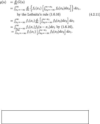
4. Functions of Random Variables and Sampling Distribution |
185 |
4.2.4 The Convolution
We start with what is also called the convolution theorem. This result will sometimes help to derive the distribution of sums of independent random variables. In this statement, we assume that the support of (X1, X2) is 2. When the support is a proper subset of 2, the basic result would still hold except that the range of the integral on the rhs of (4.2.9) should be appropriately adjusted on a case by case basis.
Theorem 4.2.1 (Convolution Theorem) Suppose that X1 and X2 are independent continuous random variables with the respective pdf’s f1(x1) and f2(x2), for (x1, x2) 2. Let us denote U = X1 + X2. Then, the pdf of U is given by
for u .
Proof First let us obtain the df of the random variable U. With u , we write
Thus, by differentiating the df G(u) from (4.2.10) with respect to u, we get the pdf of U and write
which proves the result. ¢
If X1 and X2 are independent continuous random variables, then the pdf of U given by (4.2.9) can be equivalently written as  instead.
186 4. Functions of Random Variables and Sampling Distribution
Example 4.2.9 Let X1 and X2 be independent exponential random variables, with their respective pdf’s given by f1(x1) = e–x1I(x1 +)
and f2(x2) = e–x2I(x2 +). What is the pdf of U = X1 + X2? It is obvious that the pdf g(u) will be zero when u ≤ 0, but it will be positive when
u > 0. Using the convolution theorem, for u > 0, we can write
which coincides with the gamma pdf in (1.7.20) with α = 2 and β = 1. In other words, the random variable U is distributed as Gamma(2, 1). See the related Exercise 4.2.19. !
A result analogous to the Theorem 4.2.1 for the product of two continuous independent random variables X1 and X2 has been set aside as the Exercise 4.2.13.
Example 4.2.10 Suppose that X1 and X2 are independent standard normal random variables with the respective pdf’s f1(x1) = (x1) and f2(x2) = (x2) for (x1, x2) 2. What is the pdf of U = X1 + X2? It is obvious that the pdf g(u) will be positive for all u . Using the convolution theorem, we can write Now, we can simplify the expression of
g(u) as follows:
where we let |
But, note that for fixed u, the function |
|
h(x) is the pdf of a N(1/2u, 1/2) variable. Thus, |
must be one. |
|
Hence, from (4.2.12), we can claim that |
for u . But, |
|
g(u) matches with the pdf of a N(0, 2) variable and hence U is distributed as N(0, 2). See the related Exercise 4.2.11. !
In the next example, X1 and X2 are not independent but the convolution or the distribution function approach still works.
Example 4.2.11 Suppose that X1 and X2 have their joint pdf given by
What is the pdf of U = X1 – X2? We first obtain the df G(u) of U.

4. Functions of Random Variables and Sampling Distribution |
187 |
Obviously, G(u) = 0 for u ≤ 0 or u ≥ 1. With 0 < u < 1, we write
Thus, the pdf of U is given by
We leave out some of the intermediate steps as the Exercise 4.2.12. !
The convolution approach leads to the distribution of U = X1 + X2 where X1, X2 are iid Uniform(0, 1). The random variable U is often said to have the triangular distribution. See the Exercise 4.2.9.
4.2.5 The Sampling Distribution
Suppose that we consider a large population of all adult men in a city and we wish to gather information regarding the distribution of heights of these individuals. Let Xj stand for the height of the jth individual selected randomly from the whole population, j = 1, ..., n. Here, n stands for the sample size. Since the population is large, we may assume from a practical point of view, that these n individuals are selected independently of each other. The simple random sampling with replacement (see the Example 1.7.6) would certainly generate independence. What is the sampling distribution of, say, the sample mean,  ? How can we proceed to understand what this theoretical distribution of may possibly mean to us in real life? A simple minded approach may consist of randomly selecting n individuals from the relevant population and record each individual’s height. The data would look like n numbers X1,1, ..., X1,n which will give rise to an observed value , namely
From the same population, if we contemplate selecting another batch of n individuals, drawn independently from the first set, and record their heights, we will end up with another data of n numbers x2,1, ..., x2,n leading to another observed value of the sample mean  , namely
Thoughwedonotphysically havetogothroughthisprocessofindependentresampling with the same sample of size n, we may think of such a hypothetical process of the identical replication, infinitely many times. Through these replications, we will finally

188 4. Functions of Random Variables and Sampling Distribution
arrive at the specific observed values  i = 1, 2, ... for the sample mean
 based on a sample of size n. In real life, however, it will be impossible to replicate the process infinitely many times, but suppose instead that we replicate one hundred times thereby coming up with the observed values
 i = 1, 2, ..., 100. One can easily draw a relative frequency histogram for this data consisting of the observed values
  i = 1, 2, ..., 100. The shape of this histogram will give us important clues regarding the nature of the theoretical distribution of the sample mean,
  . If we generated more than one hundred
  values, then the observed relative frequency histogram and the true pmf or pdf of
  would have more similarities. With this perception of the independent resampling again and again, the adjective “sampling” is attached when we talk about the “distribution” of
  . In statistical applications, the sample mean frequently arises and its theoretical distribution, as told by its pmf or the pdf, is customarily referred to as the sampling distribution of
  . In the same vein, one can think about the sampling distributions of many other characteristics, for example, the sample median, sample standard deviation or the sample maximum in a random sample of size n from an appropriate population under consideration. In practice, for example, it is not uncommon to hear about the sampling distribution of the median income in a population or the sampling distribution of the record rainfall data in a particular state over a period. We would use both phrases, the sampling distribution and distribution, quite interchangeably.
Example 4.2.12 (Example 4.2.4 Continued) Let X be a random variable with its pdf
Now, suppose that we wish to select 1000 random samples from this population. How can we accomplish this? Observe that the df of X is
and we know that F(X) must be distributed as the Uniform(0, 1) random variable. Using the MINITAB Release 12.1 and its uniform distribution gen-
erator, we first obtain 1000 observed values u1, u2, ..., u1000 from the Uniform(0, 1) distribution. Then, we let
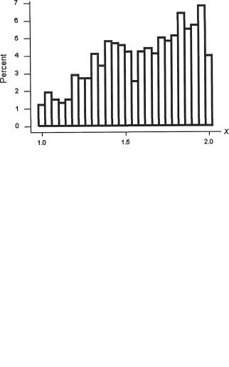
4. Functions of Random Variables and Sampling Distribution |
189 |
Figure 4.2.1. The Histogram of 1000 Sample Values Drawn According to the PDF f(x) from (4.2.13)
These xi’s form a random sample of size 1000 from a population with its pdf f(x) given by (4.2.13). Next, using the MINITAB Release 12.1, a histogram
was constructed from these 1000 sample values x1, x2, ..., x1000 which is presented in the Figure 4.2.1. This histogram provides a sample-based picture
approximating the true pdf given by (4.2.13).
Figure 4.2.2. The Plot of the PDF f(x) from (4.2.13)
In this situation, we know the exact form of the pdf f(x) which is plotted between –0.5 and 2.5 in the Figure 4.2.2 with the help of MINITAB, Release 12.1. Visual examinations reveal that there are remarkable similarities between the histogram from the Figure 4.2.1 and the plot of f(x) from the Figure 4.2.2. In practice, a sample-based histogram is expected to be a good approximation of the population distribution, particularly if the sample size is not too small. !
190 4. Functions of Random Variables and Sampling Distribution
4.3 Using the Moment Generating Function
The moment generating function (mgf) of a random variable was introduced in the Section 2.3. In the Section 2.4 we had emphasized that a finite mgf indeed pinpoints a unique distribution (Theorem 2.4.1). The implication we wish to reinforce is that a finite mgf corresponds to the probability distribution of a uniquely determined random variable. For this reason alone, the finite mgf’s can play important roles in deriving the distribution of functions of random variables.
One may ponder over what kinds of functions of random variables we should be looking at in the first place. We may point out that in statistics one frequently faces the problem of finding the distribution of a very special type of function, namely a linear function of independent and identically distributed (iid) random variables. The sample mean and its distribution, for example, fall in this category. In this vein, the following result captures the basic idea. It also provides an important tool for future use.
Theorem 4.3.1 Consider a real valued random variable Xi having its mgf MXi (t) = E(etXi) for i = 1, ..., n. Suppose that X1, ..., Xn are independent. Then, the mgf of  is given by
  where a1, ..., an are any arbitrary but otherwise fixed real numbers.
Proof The proof merely uses the Theorem 3.5.1 which allows us to split the expected value of a product of n independent random variables as the product of the n individual expected values. We write
which completes the proof. ¢
First, find the mgf MU(t). Visually match this mgf with that of one of the standard distributions. Then, U has that same distribution.
A simple looking result such as the Theorem 4.3.1 has deep implications. First, the mgf MU(t) of U is determined by invoking Theorem 4.3.1. In view of the Theorem 2.4.1, since the mgf of U and the distribution of U correspond uniquely to each other, all we have to do then is to match the form of this mgf MU(t) with that of one of the standard distributions. This way we will identify the distribution of U. There are many situations where this simple approach works just fine.
4. Functions of Random Variables and Sampling Distribution |
191 |
Example 4.3.1 (Example 4.2.3 Continued) Let X1, ..., Xk be independent and let Xi be Binomial(ni, p), i = 1, ..., k. Write  Then invoking Theorem 4.3.1 and using the expression of the mgf of the Binomial (ni, p) random variable from (2.3.5),
one has The final expression of MU(t) matches with the expression for the mgf of the Binomial (n, p) random variable found in (2.3.5). Thus, we can claim that the sampling distribution of U is Binomial with parameters n and p since the correspondence between a distribution and its finite mgf is unique. !
Example 4.3.2 Suppose that we roll a fair die n times and let Xi denote the score, that is the number on the face of the die which lands upward on the ith toss, i = 1, ..., n. Let  the total score from the n tosses. What is the probability that U = 15? The technique of full enumeration will be very tedious. On the other hand, let us start with the mgf of any of the Xi’s which
is given by MXi(t) = 1/6et (1 + et + ... + e5t) and hence MU(t) = 1/6nent (1 + et +
... + e5t)n. In the full expansion of MU(t), the coefficient of ekt must coincide with P(X = k) for k = n, n + 1, ..., 6n–1, 6n. This should be clear from the way the mgf of any discrete distribution is constructed. Hence, if n = 4, we have P(X = 15) = 1/64{coefficient of e11t in the expansion of (1 + et + ... + e5t)10} = 140/64} = But, if n = 10, we have P(X = 15) = 1/610{coefficient of e5t in the expansion of (1 + et + ... + et)4} = 2002/610. One can find the pmf of U as an exercise. !
Example 4.3.3 Let X1, ..., Xn be independent random variables, Xi distributed as  i = 1, ..., n. Write
  and
and  Then invoking Theorem 4.3.1 and using the expression for the mgf of the
  random variable from (2.3.16), one has
  The final ex-
pression of MU(t) matches with the expression for the mgf of the N(µ, σ2) random variable found in (2.3.16). Thus, we can claim that the sampling distribution of U is normal with parameters µ and σ2 since the correspondence between a distribution and its finite mgf is unique. !
Example 4.3.4 Let X1, ..., Xn be independent random variables, Xi having a |
|
Gamma distribution with the pdf fi(x) = cie–x/βxαi–1 with |
|
for 0 < x, αi, β < ∞, i = 1, ..., n. Let us write U = |
Then, for 0 < |
t < β–1, as before one has M (t) = |
|
U |
|
Here we used the expression for the mgf of the Gamma(αi, β) random variable from (2.3.23). Thus, we can claim that the sampling distribution of U is Gamma(α,
β) since the correspondence between a distribution and its finite mgf is unique. ! Example 4.3.5 Let X1, ..., Xn be independent random variables, Xi be
192 4. Functions of Random Variables and Sampling Distribution
distributed as N(µi,  ), i = 1, ..., n. With fixed but otherwise arbitrary real numbers a1, ..., an, we write
  and then denoting
  and
and  we claim along the lines of the Example 4.3.3 that the sampling distribution of U turns out to be N(µ, σ2). It is left as the Exercise 4.3.3.!
For the record, we now state the following results. Each part has already been verified in one form or another. It will, however, be instructive to supply direct proofs using the mgf technique under these special situations. These are left as the Exercise 4.3.8.
Theorem 4.3.2 (Reproductive Property of Independent Normal, Gamma and Chi-square Distributions) Let X1, ..., Xn be independent random variables. Write  and
and  = n–1U. Then, one can conclude the following:
(i)If Xi’s have the common N(µ, σ2) distribution, then U is distributed as N(nµ, nσ2) and hence  is distributed as N(µ, 1/nσ2);
(ii)If Xi’s have the common Gamma (α, β) distribution, then U is dis tributed as Gamma(nα, β);
(iii)If Xi has a Gamma(½νi, 2) distribution, that is a Chi-square distri
bution with νi degrees of freedom for i = 1, ..., n, then U is distrib
uted as Gamma(½ν, 2) with |
which is a Chi-square |
distribution with ν degrees of freedom.
Example 4.3.6 (Example 4.1.1 Continued) Now, let us briefly go back to the Example 4.1.1. There, we had Z1, Z2 iid N(0, 1) and in view of the Example 4.2.6 we can claim that are iid  . Thus, by using the reproductive property of the independent Chi-squares, we note that the random variable
  is distributed as the
  random variable. The pdf of W happens to be g(w) = 1/2e–w/2I(w > 0). Hence, in retrospect, (4.1.4) made good sense. !
4.4 A General Approach with Transformations
This is a more elaborate methodology which can help us to derive distributions of functions of random variables. We state the following result without giving its proof.
Theorem 4.4.1 Consider a real valued random variable X whose pdf is f(x) at the point x belonging to some subinterval χ of the real line . Suppose that we have a one-to-one function g: χ → and let g(x) be differentiable with respect to x( χ). Define the transformed random variable

4. Functions of Random Variables and Sampling Distribution |
193 |
Y = g(X). Suppose that the domain space  of Y is also a subinterval of . Then, the pdf of Y is given by
for y γ.
That is, in the expression of f(x), the x variable is first replaced by the new variable g–1(y) everywhere and then we multiply the resulting expression by the abso-
lute value of the Jacobian of transformation which is |
Incidentally, note |
|
that |
is evaluated as the absolute value of dx/dy and then replacing |
|
the variable x χ in terms of the new variable Y  .
.
Figure 4.4.1. A Mapping of x to y
Recall the convention that when a pdf is written down with its support, it is understood that the densitY is zero elsewhere.
Example 4.4.1 (Example 4.2.5 Continued) We write W = F(X) where we have g(x) = F(x) for x (a, b), so that x = F–1(w) for w for w (0, 1). This transformation from x to w is one-to-one. Now, dw/dx = f(x) = f(F–1(w)). Then, using (4.4.1) the pdf of W becomes
In other words, W = F(X) is distributed uniformly on the interval (0, 1). Next, we have U = q(W) where q(w) = –log(w) for 0 < w < 1. This transformation from w to u is also one-to-one. Using (4.4.1) again, the pdf of U is obtained as follows:
which shows that U is distributed as a standard exponential variable or Gamma(1, 1). !
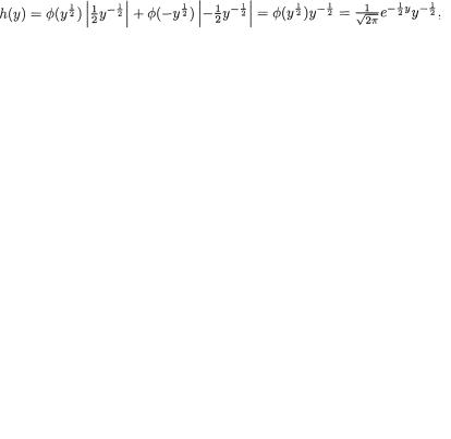
194 4. Functions of Random Variables and Sampling Distribution
Example 4.4.2 Let U be a Uniform(0, 1) variable, and define V = –log(U), W = –2log(U). From the steps given in the Example 4.4.1, it immediately follows that V has the standard exponential distribution. Using (4.4.1) again, one should verify that the pdf of W is given by g(w) = 1/2e–w/2I(w > 0) which coincides with the pdf of a Chi-square random variable with 2 degrees of freedom. !
In the case when g(.) considered in the statement of the Theorem 4.4.1 is not one-to-one, the result given in the equation (4.4.1) needs some minor adjustments. Let us briefly explain the necessary modifications. We begin by partitioning the χ space into A1, ..., Ak in such a way that the individual transformation g : Ai →  becomes one-to-one for each i = 1, ..., k. That is, when we restrict the mapping g on Ai →
  , given a specific value y
  , we can find a unique corresponding x in Ai which is mapped into y, and suppose that
we denote, |
i = 1, ..., k. Then one essentially applies the Theorem |
4.4.1 on each set in the partition where gi, which is the same as g restricted on Ai →  , is one-to-one. The pdf h(y) of Y is then obtained as follows:
Example 4.4.3 Suppose that Z is a standard normal variable and Y = Z2. This transformation from z to y is not one-to one, but the two pieces of transformations from z [0, ∞) to y + and from z (–∞, 0) to y + are individually one-to-one. Also recall that the pdf of Z, namely, (z) is symmetric about z = 0. Hence, for 0 < y < ∞, we use (4.4.2) to write down the pdf h(y) of Y as follows:
which coincides with the pdf of a Chi-square variable with one degree of freedom. Recall the earlier Example 4.2.6 in this context where the same pdf was derived using a different technique. See also the Exercise 4.4.3-4.4.4.!
Example 4.4.4 Suppose that X has the Laplace or double exponential distribution with its pdf given bY f(x) = 1/2e–|x| for x . Let the transformed variable be Y = |X|. But, g(x) = |x| : → + is not one-to-one. Hence, for 0 < y < ∞, we use (4.4.2) to write down the pdf h(y) of Y as follows:
which coincides with the pdf of a standard exponential variable. See also the Exercise 4.4.5. !
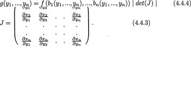
4. Functions of Random Variables and Sampling Distribution |
195 |
4.4.1 Several Variable Situations
In this subsection, we address the case of several variables. We start with the machinery available for one-to-one transformations in a general case. Later, we include an example when the transformation is not one-to-one. First, we clarify the techniques in the two-dimensional case. One may review the Section 4.8 for some of the details about matrices.
Suppose that we start with real valued random variables X1, ..., Xn and we have the transformed real valued random variables Yi = gi(X1, ..., Xn), i = 1, ..., n where the transformation from (x1, ..., xn) χ to (y1, ..., yn),  is assumed to be one-to one. For example, with n = 3, we may have on hand three
transformed random variables Y1 = X1 + X2, Y2 = X1 – X2, and Y3 = X1 + X2 +
X3.
We start with the joint pdf f(x1, ..., xn) of X1, ..., Xn and first replace all the variables x1, ..., xn appearing within the expression of f(x1, ..., xn) in terms of the transformed variables  i = 1, ..., n. In other words, since the transformation (x1, ..., xn) to (y1, ..., yn) is one-to one, we can theoreticallY think of uniquely expressing xi in terms of (y1, ..., yn) and write xi = bi(y1, ..., yn), i = 1, ..., n. Thus, f(x1, ..., xn) will be replaced by f(b1, ..., bn). Then, we multiply f(b1, ..., bn) by the absolute value of the determinant of the Jacobian matrix of transformation, written exclusively involving the transformed variables y1, ..., yn only. Let us define the matrix
The understanding is that each xi variable is replaced by bi(y1, ..., yn), i = 1, ..., n, while forming the matrix J. Let det(J) stand for the determinant of the matrix J and | det(J) | stand for the absolute value of det(J). Then the joint pdf of the transformed random variables Y1, ..., Yn is given by
for y γ.
On the surface, this approach may appear complicated but actually it is not quite so. The steps involved are explained by means of couple of examples.
Example 4.4.5 Let X1, X2 be independent random variables and Xi be distributed as Gamma(αi, β), αi > 0, β > 0, i = 1, 2. Define the transformed variables Y1 = X1 + X2, Y2 = X1/(X1 + X2). Then one can uniquely
196 4. Functions of Random Variables and Sampling Distribution
express x1 = y1y2 and x2 = y1 (1 – y2). It is easy to verify that
so that det(J) = –y1y2 – y1(1 – y2) = –y1. Now, writing the constant c instead of the expression {βα1+α2Γ(α1)Γ(α2)}–1, the joint pdf of X1 and X2 can be written as
for 0 < x1, x2 < ∞. Hence using (4.4.4) we can rewrite the joint pdf of Y1 and Y2 as
for 0 < y1 < ∞, 0 < y2 < 1. The terms involving y1 and y2 in (4.4.5) factorize and also either variable’s domain does not involve the other variable. Refer back to the Theorem 3.5.3 as needed. It follows that Y1 and Y2 are independent random variables, Y1 is distributed as Gamma(α1 + α2,β) and Y2 is distributed as Beta(α1, α2) since we can rewrite c as {βα1+α2Γ(α1 + α2)}–1 {b(α1, α2)}–1 where b(α1, α2) stands for the beta function, that is
One may refer to (1.6.19) and (1.6.25)-(1.6.26) to review the gamma and beta functions. !
Example 4.4.6 (Example 4.4.5 Continued) Suppose that X1, ..., Xn are independent random variables where Xi is Gamma(αi, β), i = 1, ..., n. In view of the Example 4.4.5, we can conclude that X1 + X2 + X3 = (X1+X2)+X3 is then
Gamma(α1+α2+α3, β) whereas X1/(X1+X2+X3) is Beta(α1, α2+α3) and these are independent random variables. Thus, by the mathematical induction one can claim
that  is Gamma
 is Beta whereas these are also distributed independently. !
In the next two examples one has X1 and X2 dependent.
Also, the transformed variables Y1 and Y2 are dependent.
Example 4.4.7 Suppose that X1 and X2 have their joint pdf given by
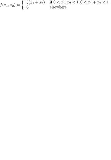
4. Functions of Random Variables and Sampling Distribution |
197 |
Let Y1 = X1 and Y2 = X1 + X2. We first wish to obtain the joint pdf of Y1 and Y2. Then, the goal is to derive the marginal pdf’s of Y1, Y2.
The one-to-one transformation (x1, x2) → (y1, y2) leads to the inverse: x1 =
y1, x2 = y2 – y1 so that |det(J)| = 1. Now, x2 > 0 implies that 0 < 2y1 < y2 < ∞ since y1 < y2 – y1. Thus, (4.4.4) leads to the following joint pdf of Y1 and Y2:
The marginal pdf’s of Y1, Y2 can be easily verified as the following:
We leave out some of the intermediate steps as the Exercise 4.4.6. Example 4.4.8 Suppose that X1 and X2 have their joint pdf given by
Let Y1 = X1 + X2 and Y2 = X1 – X2. We first wish to obtain the joint pdf of Y1 and Y2. Then, the goal is to derive the marginal pdf’s of Y1, Y2.
The one-to-one transformation (x1, x2) → (y1, y2) leads to the inverse: x1 = 1/2(y1 + y2), x2 = 1/2(y1 – y2) so that |det(J)| = 1/2. Observe that: 0 < x1 < 1
0 < y1 + y2 < 2; 0 < x2 < 1 0 < y1 – y2 < 2; 0 < x1 + x2 < 1 0 < y1 < 1. Let γ = {(y1, y2) : 0 < y1 < 1, 0 < y1 + y2 < 2, 0 < y1 – y2 < 2}. The joint pdf of Y1 and Y2 is then given by
The marginal pdf’s of Y1, Y2 can be easily verified as the following:
We leave out some of the intermediate steps as the Exercise 4.4.7. !
Example 4.4.9 The Helmert Transformation: This consists of a very special kind of orthogonal transformation from a set of n iid N(µ, σ2)

198 4. Functions of Random Variables and Sampling Distribution
random variables X1, ..., Xn, with n ≥ 2, to a new set of n random variables Y1,
..., Yn defined as follows:
Y1, ..., Yn so defined are referred to as the Helmert variables.
Let us denote the matrix
Then, one has Y = Ax where x’ = (x1, ..., xn) and y’ = (y1, ..., yn).
An×n is an orthogonal matriX. So, A’ is the inverse of A. This implies that 
In n, a sphere in the x-coordinates continues to look like a sphere in the y-coordinates when the x axes are rotated
orthogonally to match with the new y axes.
Observe that the matrix J defined in (4.4.3) coincides with the matrix A’ in the present situation and hence one can immediately write | det(J) |= | det(A’) |=| {det(AA’)}½ |= 1.
Now, the joint pdf of X1, ..., Xn is given by
for –∞ < x1, ..., xn < ∞, and thus using (4.4.4) we obtain the joint pdf of Y1, ..., Yn as follows:
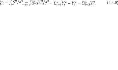
4. Functions of Random Variables and Sampling Distribution |
199 |
where –∞ < y1, ..., yn < ∞. In (4.4.8), the terms involving y1, ..., yn factorize and none of the variables’ domains involve the other variables. Thus it is clear (Theorem 3.5.3) that the random variables Y1, ..., Yn are independently distributed. Using such a factorization, we also observe that Y1 is distributed as  whereas Y2, ..., Yn are iid N(0, σ2). !
The following result plays a crucial role in many statistical analyses. IncidentallY, one should note that sometimes a population is also referred to as a universe in the statistical literature. The result we are about to mention is also indispensable in much of the distribution theory. These points will become clear in the sequel.
Theorem 4.4.2 (Joint Sampling Distribution of  and S2 from a Normal Universe) Suppose that X1, ..., Xn are iid N(µ, σ2) random variables, n ≥ 2. Define the sample mean ,
  and the sample variance
  Then, we have:
(i)The sample mean  is distributed independently of the sample variance S2;
(ii) The sampling distribution of  is and that of (n – 1)S2/ σ2 is Chi-square with (n – 1) degrees of freedom.
Proof (i) Using the Helmert transformation from (4.4.6), we can rewrite  = n–1/2 Y1. Next, observe that
using the same Helmert variables. It is clear that  is a function of Y1 alone, whereas from (4.4.9) we note that S2 depends functionallY on (Y2, ..., Yn) only. But, since Y1, ..., Yn are all independent, we conclude that
  is distributed independentlY of S2. Refer to the Theorem 3.5.2, part (ii) as needed.
(ii) Recall that |
= n–1/2 Y |
1 |
where Y is distributed as N( µ, σ2) and so |
the sampling distribution of |
1 |
||
|
follows immediately. From (4.4.9) again, it is |
||
clear that |
|
|
which is the sum of (n – 1) indepen- |
dent Chi-square random variables each having one degree of freedom. Hence, using the reproductive property of independent Chi-square variables (Theorem 4.3.2, part (iii)), it follows that (n – 1)S2/σ2 has a Chi-square distribution with (n – 1) degrees of freedom. ¢
Remark 4.4.1 Let us reconsider the setup in the Example 4.4.9 and Theorem 4.4.2. It is important to note that the sample variance S2 is the average of  and each Helmert variable independently contributes one degree of freedom toward the total (n – 1) degrees of freedom. Having n
observations X1, ..., Xn, the decomposition in (4.4.9) shows how exactly S2 can be split up into (n – 1) independent and identically distributed

200 4. Functions of Random Variables and Sampling Distribution
components. This is the central idea which eventually leads to the Analyses of Variance techniques, used so widely in statistics.
The Exercise 4.6.7 gives another transformation which proves that  and S2 are independent when the X’s are iid N(µ, σ2).
Remark 4.4.2 Let us go back one more time to the setup considered in the Example 4.4.9 and Theorem 4.4.2. Another interesting feature can be noticed among the Helmert variables Y2, ..., Yn. Only the Helmert variable Yn functionally depends on the last observed variable Xn. This particular feature has an important implication. Suppose that we have an additional observation Xn+1 at our disposal beYond X1, ..., Xn. Then, with  =
=  , the new sample variance
  and its decomposition would be expressed as
where  Here, note that Y2, ..., Yn based on X1, ..., Xn alone remain exactly same as in (4.4.6). In other words, the Helmert transformation shows exactly how the sample variance is affected in a sequential setup when we let n increase successively.
Remark 4.4.3 By extending the two-dimensional polar transformation mentioned in (4.1.2) to the n-dimension, one can supply an alternative proof of the Theorem 4.4.2. Indeed in Fisher’s writings, one often finds derivations using the n-dimensional polar transformations and the associated geometry. We may also add that we could have used one among many choices of orthogonal matrices instead of the specific Helmert matrix A given by (4.4.7) in proving the Theorem 4.4.2. If we did that, then we would be hard pressed to claim useful interpretations like the ones given in our Remarks 4.4.1-4.4.2 which guide the readers in the understanding of some of the deep-rooted ideas in statistics.
Suppose that X1, ..., Xn are iid random variables with n ≥ 2. Then,  and S2 are independent Xi’s are normally distributed.
Remark 4.4.4 Suppose that from the iid random samples X1, ..., Xn, one obtains the sample mean  and the sample variance S2. If it is then assumed that
  and S2 are independently distributed, then effectively one is not assuming anY less than normality of the original iid random variables. In other words, the independence of
  and S2 is a characteristic property of the normal distribution alone. This is a deep result in probability theory. For a proof of this fundamental characterization of a normal distribution
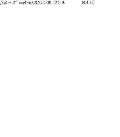
4. Functions of Random Variables and Sampling Distribution |
201 |
and other historical notes, one may refer to Zinger (1958), Lukacs (1960), and Ramachandran (1967, Section 8.3), among a host of other sources. Look at the Exercises 4.4.22-4.4.23 which can be indirectly solved using this characterization.
Example 4.4.10 The Exponential Spacings: Let X1, ..., Xn be iid with the common pdf given by
Define the order statistics Xn:1 ≤ Xn:2 ≤ ... ≤ Xn:n and let us write Yi = Xn:i, i = 1, ..., n. The Xi’s and Xn:i’s may be interpreted as the failure times and the ordered failure times respectively. Let us denote
and these are referred to as the spacings between the successive order statistics or failure times. In the context of a life-testing experiment, U1 corresponds to the waiting time for the first failure, and Ui corresponds to the time between the (i – 1)th and the ith failures, i = 2, ..., n. Here, we have a one-to- one transformation on hand from the set of n variables (y1, ..., yn) to another set of n variables (u1, ..., un). Now, in view of (4.4.4), the joint pdf of the order statistics Y1, ..., Yn is given by
Note that  . One can
also verify that | det(J) |= 1, and thus using (4.4.4) and (4.4.13), the joint pdf of U1, ..., Un can be written as
for 0 < u1, ..., un < ∞. Next, (4.4.14) can be easily rewritten as
for 0 < u1, ..., un < ∞. In (4.4.15), the terms involving u1, ..., un factorize and none of the variables’ domains involve any other variables. Thus it is clear (Theorem 3.5.3) that the random variables U1, ..., Un are independently distributed. Using such a factorization, we also observe that Ui has an exponential distribution with the mean (n – i + 1)–1β,i = 1, ..., n. !

202 4. Functions of Random Variables and Sampling Distribution
Example 4.4.11 (Example 4.4.10 Continued) Suppose that the X’s are iid and the common pdf is the same as the one in (4.4.11). For all k = 1, ..., n – 1, observe that
z
and hence
Since  we have
It is worthwhile to note that we have succeeded in deriving an expression for the expected value of the kth order statistic Xn:k without finding the marginal distribution of Xn:k. These techniques are particularly useful in the areas of reliability and survival analyses. !
If the X’s are iid normal, the Helmert transformation provides a natural way to consider intricate properties of  and S2. If the X’s are iid exponential or negative exponential, the transformation involving the spacings between the successive order statistics is a natural one to consider instead.
Example 4.4.12 The Negative Exponential Distribution: Suppose that
X1, ..., Xn are iid random variables having a common pdf given by
where µ is the location parameter and σ is the scale parameter. In reliability applications, is often referred to as the minimum guarantee time or the minimum threshold, and hence is assumed positive in such applications. Refer back to (1.7.36) as needed. We will, however, continue to assume that µ is an arbitrary real number. Let us consider the two random variables
and look at their distributions. Denote Wi = Xi – µ and then it is clear that W1, ..., Wn are iid having the common pdf given by in (4.4.11) with β replaced by σ. Following the Example 4.4.10, we write U1 = Wn:1, U2 =

4. Functions of Random Variables and Sampling Distribution |
203 |
Wn:2 – Wn:1, ..., Un = Wn:n – Wn:n–1, and realize that n(Xn:1 – µ)/σ is same as nU1/σ, which has the standard exponential distribution. That is, n(Xn:1 – µ)/σ
is distributed as the standard exponential distribution which is the same as Gamma (1, 1). Also, recall that U1, ..., Un must be independent random variables. Next, one notes that
Now, it is clear that T is distributed independently of Xn:1 because T functionally depends only on (U2, ..., Un) whereas Xn:1 functionally depends only on U1. But, U1 is independent of (U2, ..., Un). Also, note that
where Z2n, ..., Znn are iid random variables having the Chi-square distribution with two degrees of freedom. Thus, using the reproductive property of independent Chi-square variables (Theorem 4.3.2, part (iii)), we conclude that has the Chi-square distribution with 2(n – 1) degrees of
freedom. !
Suppose that X1, ..., Xn are iid random variables.
If their common distribution is negative exponential, then
Xn:1 and  are independent.
Remark 4.4.5 If we compare (4.4.20) with the representation given in (4.4.9), it may appear that in principle, the basic essence of the Remark 4.4.1 holds in this case too. It indeed does, but only partially. One realizes fast that in the present situation, one is forced to work with the spacings between the successive order statistics. Thus, the decomposition of 2Tσ–1 into unit independent components consists of (n – 1) random terms, each depending on the sample size n. This is fundamentally different from what we had observed in (4.4.9) and emphasized earlier in the Remark 4.4.2.
In the next example X1 and X2 are independent, but the transformed variables Y1 and Y2 are dependent.
Example 4.4.13 (Example 4.4.5 Continued) Suppose that X1 and X2 are iid standard exponential random variables. Thus,

204 4. Functions of Random Variables and Sampling Distribution
We denote y1 = x1 + x2, y2 = x2 so that for this one-to-one transformation we
have x1 = y1 – y2, x2 = y2 where 0 < y2 < y1 < ∞. One can verify that | det(J) | = 1, and hence the joint pdf of Y1 and Y2 would become
Then, from (4.4.21) we obtain the marginal pdf of Y1 as
In other words, Y1 = X1 + X2 has the Gamma(2, 1) distribution. We leave out the intermediate steps as the Exercise 4.4.16. !
In the next example X1, X2 and X3 are independent, but the transformed variables Y1, Y2 and Y3 are dependent.
Example 4.4.14 (Example 4.4.13 Continued) Suppose that X1, X2 and X3 are iid standard exponential random variables. Thus,
We denote y1 = x1 + x2 + x3, y2 = x2, y3 = x3 so that for this one-to-one transformation we have x1 = y1 – y2 – y3, x2 = y2, x3 = y3 where 0 < y2 < y1 ∞, 0 < y3 < y1 < ∞ and y2 + y3 < y1. One can verify that | det(J) | = 1, and hence the joint pdf of Y1, Y2 and Y3 would become
Then, from (4.4.22) we obtain the marginal pdf of Y1 as
In other words, Y1 = X1 + X2 + X3 has the Gamma(3, 1) distribution. We leave out the intermediate steps as the Exercise 4.4.17. !
In the next example X1 and X2 are dependent, but the transformed variables Y1 and Y2 are independent.
Example 4.4.15 Suppose that the random vector (X1, X2) has the bivariate normal distribution, N2(0, 0, σ2, σ2, ρ) with 0 < σ < ∞, –1 < ρ < 1.
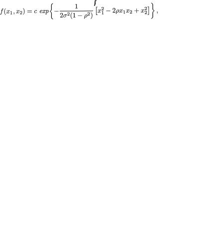
4. Functions of Random Variables and Sampling Distribution |
205 |
Let us derive the joint pdf of Y1 = X1 + X2 and Y2 = X1 – X2. Refer to the Section 3.6 as needed. With c = {2πσ2(1 – ρ2)–1/2}–1, we start with
where –∞ < x1, x2 < ∞. For the one-to-one transformation on hand, we have
x1 = 1/2(y1 + y2), x2 = 1/2(y1 – y2) with 0 < y1, y2 < ∞. One can easily verify that | det(J)| = 1/2, and hence the joint pdf of Y1 and Y2 would become
for –∞ < y1, y2 < ∞. In (4.4.23), the terms involving y1, y2 factorize and none of the variables’ domains involve the other variable. Thus it is clear (Theorem 3.5.3) that the random variables Y1, Y2 are independently distributed. Using such a factorization, we also observe that Y1 = X1 + X2 is distributed as N(0, 2σ2(1 + ρ)) whereas Y2 = X1 – X2 is distributed as N(0, 2σ2(1 – ρ)). !
Suppose that the transformation from (X1, ..., Xn) → (Y1, ..., Yn) is not one-to-one. Then, the result given in the equation (4.4.4) will need slight adjustments. Let us briefly explain the necessary modifications. We begin by partitioning the χ space, that is the space for (x1, ..., xn), into A1, ..., Ak in such a way that the associated transformation from Ai → y, that is the space for (y1, ..., yn), becomes separately one-to-one for each i = 1, ..., k. In other words, when we restrict the original mapping of (x1, ..., xn) → (y1, ..., yn) on
Ai → y, given a specific (y1, ..., yn) y, we can find a unique (x1, ..., xn) in Ai which is mapped into (y1, ..., yn). Given (y1, ..., yn), let the associated xj =
bij(y1, ..., yn), j = 1, ..., n, i = 1, ..., k. Suppose that the corresponding Jacobian matrix is denoted by Ji, i = 1, ..., k. Then one essentially applies (4.4.4) on each piece A1, ..., Ak and the pdf g(y1, ..., yn) of Y is obtained as follows:
for y y. For a clear understanding, let us look at the following example.
Example 4.4.16 Suppose that X1 and X2 are iid N(0, 1) variables. Let us denote Y1 = X1/X2 and Y2 =  Obviously, the transformation (x1, x2) → (y1, y2) is not one-to-one. Given (y1, y2), the inverse solution would be
  or
or  We should take A1 = {(x1, x2) 2 : x2 > 0}, A2 = {(x1, x2) 2 : x2 < 0}. Now, we apply
206 4. Functions of Random Variables and Sampling Distribution
(4.4.24) directly as follows: With –∞ < y1 < ∞, 0 < y2 < ∞, we get
With –∞ < y1 < ∞ and the substitution  the marginal pdf g1(y1) of Y1 is then obtained from (4.4.25) as
which coincides with the Cauchy pdf defined in (1.7.31). That is, X1/X2 has the Cauchy distribution. 
Next, with the substitution
∞, the marginal pdf g2(y2) of Y2 is then obtained from (4.4.25) as
But, note that h(y1) resembles the pdf of the  variable for any fixed
0 < y2 < ∞. Hence, |
must be one for any fixed 0 < y2 < ∞. |
That is, for all fixed 0 < y2 < ∞, we get
which coincides with the pdf of the x12 variable. In other words, has the  distribution. !
The Exercise 4.4.18 provides a substantial generalization in the sense that X1/X2 can be claimed to have a Cauchy distribution even when (X1, X2) has the N2(0, 0, σ2, σ2, ρ) distribution. The transformation used in the Exercise 4.4.18 is also different from the one given in the Example 4.4.16.
4.5 Special Sampling Distributions
In the Section 1.7, we had listed some of the standard distributions by including their pmf or pdf. We recall some of the continuous distributions,
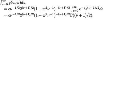
4. Functions of Random Variables and Sampling Distribution |
207 |
particularly the normal, gamma, Chi-square, Student’s t, the F and beta distributions. At this point, it will help to remind ourselves some of the techniques used earlier to find the moments of normal, Chi-square or gamma variates.
In this section, we explain how one constructs the Student’s t and F variables. Through examples, we provide some justifications for the importance of both the Student’s t and F variates. When we move to the topics of statistical inference, their importance will become even more convincing.
4.5.1The Student’s t Distribution
Definition 4.5.1 Suppose that X is a standard normal variable, Y is a Chisquare variable with í degrees of freedom, and that X and Y are independently
distributed. Then, the random variable  is said to have the Student’s t distribution, or simply the t distribution, with í degrees of freedom.
Theorem 4.5.1 The pdf of the random variable W mentioned in the Definition 4.5.1, and distributed as tí, is given by
with
Proof The joint pdf of X and Y is given by
for –∞ < x < ∞, 0 < y < ∞ where  Let us denote u
= y and |
so that the inverse transformation is given by |
 and y = u. Note that
  From (4.5.1), the joint pdf of U and W can be written as
for 0 < u < ∞, –∞ < w < ∞. Thus, for –∞ < w < ∞ and with the substitution s = u(1 + w2ν–1)/2, the pdf h(w) of W is given by
which matches with the intended result. Some of the details are left out as the Exercise 4.5.1.¢
208 4. Functions of Random Variables and Sampling Distribution
Once the pdf h(w) is simplified in the case ν = 1, we find that h(w) = π–1 (1+w2)–1 for –∞ < w < ∞. In other words, when ν = 1, the Student’s t distribution coincides with the Cauchy distribution. Verification of this is left as the Exercise 4.5.2.
In some related problems we can go quite far without looking at the pdf of the Student’s t variable. This point is emphasized next.
A case in point: note that –W thus defined can simply be written as  Since (i) –X is distributed as standard normal, (ii) –X is distributed independently of Y, we can immediately conclude that W and –W have identical distributions, that is the Student’s t distribution is symmetric around zero. In other words, the pdf h(w) is symmetric around w = 0. To conclude this, it is not essential to look at the pdf of W. On the other hand, one may arrive at the same conclusion by observing that the pdf h(w) is such that h(w) = h(–w) for all w > 0.
How about finding the moments of the Student’s t variable? Is the pdf h(w) essential for deriving the moments of W? The answer is: we do not really need it. For any positive integer k, observe that
as long as E[Y–k/2] is finite. We could split the expectation because X and Y are assumed independent. But, it is clear that the expression in (4.5.2) will lead to finite entities provided that appropriate negative moments of a Chi-square variable exist. We had discussed similar matters for the gamma distributions in (2.3.24)-(2.3.26).
By appealing to (2.3.26) and (4.5.2), we claim that for the Student’s t variable W given in the Definition 4.5.1, we have E(W) finite if 1/2ν > –(–1/2) that is if ν > 1, whereas E(W2) is finite, that is V(W) is finite when 1/2ν > –(– 1) or ν > 2. One should verify the following claims:
and also,
Example 4.5.1 The One-Sample Problem: Suppose that X1, ..., Xn are iid N(µ, σ2), –∞ < µ < ∞, 0 < σ < ∞, n ≥ 2. Let us recall that  is
is
distributed as N(0, 1), (n – 1)S2/σ2 is  and these two are also independent (Theorem 4.4.2). Then, we rewrite

4. Functions of Random Variables and Sampling Distribution |
209 |
In other words,  has the same representation as that of W with ν = n – 1. Hence, we can claim that
A standardized variable such as |
is widely used in the sequel |
when the population mean µ and variance σ2 are both unknown.
W. S. Gosset was a pioneer in the development of statistical methods for design and analysis of experiments. He is perhaps better known under the pseudonym “Student” than under his own name. In most of his papers, he preferred to use the pseudonym “Student” instead of his given name. His path-breaking 1908 paper gave the foundation of this t-distribution. !
Example 4.5.2 The Two-Sample Problem: Suppose that the random vari-
ables Xi1, ..., Xini are iid N(µi, σ2), i = 1, 2, and that the X1j’s are independent of the X2j’s. With ni ≥ 2, let us denote
for i = 1, 2.

 is called the pooled sample variance.
Now,  2, and these are also independent. Using the reproductive property of independent Chi-squares (Theorem 4.3.2,
part (iii)) we claim that  has a Chi-square dis-
tribution with (n1 + n2 – 2) degrees of freedom. Also,  and
and  are independent. Along the lines of the Example 4.5.1, we can claim that
This two-sample Student’s t distribution is widely used in the statistical literature. !
4.5.2 The F Distribution
Definition 4.5.2 Let X, Y be independent Chi-square random variables distributed respectively with í1 and í2 degrees of freedom. Then, the random variable U = (X/ ν1) ÷ (Y/ ν2) is said to have the F distribution with degrees of freedom ν1, ν2, in that order.
210 4. Functions of Random Variables and Sampling Distribution
Theorem 4.5.2 The pdf of the random variable U mentioned in the Definition 4.5.2, and distributed as Fí1, í2, is given by
with k = k(ν1, ν2) = (ν1/ν2)1/2ν1 Γ((ν1 + ν2)/2) {Γ(ν1/2)Γ(ν2/2)}–1 and ν1, ν2 = 1, 2, ... .
Proof The joint pdf of X and Y is given by
for 0 < x, y < ∞ where c = {2(ν1+ν2)/2Γ(ν1/2)Γ(ν2/2)}–1. Let us denote u = νν2-1 x/y and v = y, so that the inverse transformation is given by x = νν-12 uv and y = v. Note that |J| = νν-12v. From (4.5.9), the joint pdf of U and V can be written as
for 0 < u, v < ∞. Thus, for 0 < u < ∞, the pdf h(u) of U is given by
by viewing the integrand as a gamma pdf, which matches with the intended result. ¢
In some related problems we can go quite far without looking at the pdf of the F variable. This point is emphasized next.
From the Definition 4.5.1 of the Student’s t random variable W, it is clear that W2 = X2(Y/ν)–1. Since (i) X2, Y are distributed as Chi-squares respectively with one and ν degrees of freedom, (ii) X2 and Y are also independent, we can conclude that W2 has the same form as in the Definition 4.5.2 for U. Thus, the pdf of U is not essential to arrive at the conclusion:

 has the same distribution as that of F1, ν
The F distribution is not symmetric in the same sense as the t distribution is. But, from the Definition 4.5.2, it follows immediately though that 1/U, which is the same as (Y/ ν2) ÷ (X/ ν1), should be distributed
4. Functions of Random Variables and Sampling Distribution |
211 |
as Fν2, ν1. That is, 1/F has a F distribution too. This feature may be intuitively viewed as the “symmetry property” of the pdf h(u). The explicit form of the pdf has not played any crucial role in this conclusion.
How about finding the moments of the Fν1, ν2 variable? The pdf h(u) is not essential for deriving the moments of U. For any positive integer k, observe that
as long as E[Y–k] is finite. We can split the expectation in (4.5.10) because X and Y are assumed independent. But, it is clear that the expression in (4.5.10) will lead to finite entities provided that appropriate negative moment of a Chisquare variable exists. We had discussed similar matters for the gamma distributions in (2.3.24)-(2.3.26).
By appealing to (2.3.26) and (4.5.10), we claim that for the Fν1, ν2 variable given in the Definition 4.5.2, we have E(U) finite if ν2 > 2, whereas E(U2) is finite, that is V(U) is finite when ν2 > 4. One should verify the following claims:
and also
Example 4.5.3 The Two-Sample Problem: Let Xi1, ..., Xini be iid
 i = 1, 2, and that the X1j’s are independent of the X2j’s. For ni ≥ 2, we denote
  as in the
Example 4.5.2. Now, , (ii) they are also independent, and hence in view of the Definition 4.5.2, the random variable U = (S1/σ1)2 ÷ (S2/σ2) has the F distribution with degrees of freedom ν1 = n1 – 1, ν2 = n2 – 1. !
4.5.3 The Beta Distribution
Recall the random variable U mentioned in the Definition 4.5.2. With k = k(ν1,ν2) = (ν1/ν2)1/2 ν1 Γ((ν1 + ν2)/2) {Γ(ν1/2)Γ(ν2/2)}–1, the pdf of U was
for 0 < u < ∞. Now, let transformation from u →
us define Z = [(ν1/ν2)U]/[1 + (ν1/ν2)U]. The z is one-to-one and we have (ν1/ν2)u = z(1 –
212 4. Functions of Random Variables and Sampling Distribution
z)–1, 0 < u < ∞, 0 < z < 1. One may also check that (ν /ν ) du- = (1 – z)–2. Thus,
1 2 dz
combining (4.4.1) and (4.5.13) in a straightforward fashion, we can write down the pdf of Z as follows: For 0 < z < 1, we have
which simplifies to
It coincides with the beta pdf defined in (1.7.35) where α = 1/2ν1 and β = 1/ 2ν2. That is,
[(ν1/ν2)Fν1, ν2]/[1 + (ν1/ν2) Fν1, ν2] has Beta (1/2ν1, 1/2ν2) distribution.
4.6 Special Continuous Multivariate Distributions
We now include some interesting aspects of the multivariate normal, t, and F distributions. It will become clear shortly that both the multivariate t and F distributions are close associates of the multivariate normal distribution. One may review the Section 4.8 for some of the details about matrices.
Tong’s (1990) book is devoted to the multivariate normal distributions and includes valuable tables. It briefly discusses the multivariate t and F distributions too. The references to the tables and other features for the multivariate normal, t and F distributions can be found in Johnson and Kotz (1972).
We included important properties of a bivariate normal distribution in the Section 3.6. The sampling distributions in the context of a bivariate normal population, however, is included in the present section.
4.6.1 The Normal Distribution
The bivariate normal density was given in (3.6.1). The general multivariate normal density is more involved. But, without explicitly referring to the pdf, one can derive many interesting and useful properties. The following broad definition of the p-dimensional normality can be found in Rao (1973, p. 518.) The advantage of adopting this definition over another relying explicitly on the multivariate pdf will be clear from the Examples 4.6.1-4.6.2.
Definition 4.6.1 A p(≥ 1) random vector X = (X1, ..., Xp) is said to have a p-dimensional normal distribution, denoted by Np, if and only if
4. Functions of Random Variables and Sampling Distribution |
213 |
each linear function |
|
|
|
|
|
has the univariate normal distribution for all |
||||||||||
fixed, but arbitrary real numbers a1, ..., ap. |
|
|
|
|
|
|
|
|||||||||
|
Example 4.6.1 Suppose that X , ..., X are iid N (µ, σ2), –∞ < µ < ∞, 0 < |
|||||||||||||||
|
|
|
|
|
|
|
|
1 |
n |
|
|
|
|
|
|
|
σ < ∞. Consider the sample mean |
and let us look at the two-dimensional |
|||||||||||||||
joint |
distribution |
of |
(X |
1 |
, |
). |
Obviously, |
E(X |
1 |
)=E( )=µ,V(X |
1 |
) |
||||
=σ |
2 |
and V( ) |
= |
1 |
2 |
|
Also, we can |
|
|
|
, ) |
|
||||
|
-σ |
|
. |
|
write Cov(X |
1 |
= |
|||||||||
|
|
|
|
n |
|
|
|
|
|
|
|
|
|
|
|
|
|
|
|
|
|
|
|
|
|
Refer to the Theorem 3.4.3, |
|||||||
part (iii) as needed. But, the covariance between X1 and Xj is zero for 1 < j ≤
1 |
1 |
2 |
and hence |
Any |
n. That is, Cov(X1, ) = n- Cov(X1, X1) = n-σ |
|
|||
linear function L of X1 and |
is also a linear function of n original iid normal |
|||
random variables X1, ..., Xn, and hence L itself is distributed normally. This follows from the reproductive property of independent normal variables (Theorem 4.3.2, part (i)). So, by the Definition 4.6.1 it follows that (X1,  ) is jointly distributed as a bivariate normal variable. Thus, the conditional distri-
bution of X |
given |
is |
is N ( , σ2 (1 – 1/n)) which provides the |
||
|
1 |
|
and V(X1 | |
2 |
1 |
following facts: |
|
||||
|
) = σ |
(1 – n-). Refer |
|||
to the Theorem 3.6.1 as needed. Look at the Exercise 4.6.1 !
Example 4.6.2 (Example 4.6.1 Continued) One can easily find the condi-
tional expectation of aX1 + bX2 |
given |
|
|
in the following way where a |
||
and b are fixed non-zero real numbers. Observe that E(aX1 + bX2 | |
) |
|||||
= E(aX1 | |
) + E(bX2 | |
) = (a + b) . Also note, for example, that |
||||
|
= V(X | |
) + {E(X |
1 |
| |
)}2 = σ2(1 – 1/n) + 2 . |
|
|
1 |
|
|
|
|
|
One can exploit similar techniques to obtain other expected values in this context. Look at the Exercise 4.6.2. !
Example 4.6.3 (Example 4.6.1 Continued) A result such as E(X1| |
|||||
= can be alternately derived as follows. Obviously,E(X1 | |
) = , and |
||||
this can be rewritten as |
|
|
|
) |
|
E(X1 | |
) which was the intended result in the first place. This argument |
||||
works here because E{Xi | |
} = E(X1 |
| |
) for each i = 1, ..., n. |
||
Observe that this particular approach merely used the fact that the Xi’s are iid, |
|||||
but it did not exploit the fact that the Xi’s are iid normal to begin with. ! |
|||||
Example 4.6.4 (Example 4.6.2 Continued) A result such as |
|||||
|
) = σ2(1 – 1/n) + 2 can be alternately derived as follows. Obviously, |
||||
σ2 = E(S2) = E(S2 | |
) since S2 and |
are independent. Here, we have |
|||
indeed used the full power of the assumption of normality. Recall the Remark 4.4.4 in this context. So one can write and hence
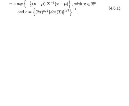
214 4. Functions of Random Variables and Sampling Distribution
 } =
} =  + (n – 1)σ2. This leads to the desired conclusion:
 } =
} =  + (1 – 1/n)σ2.
For completeness, we now give the pdf of the p-dimensional normal random vector. To be specific, let us denote a p-dimensional column vector X whose transpose is X’ = (X1, ..., Xp), consisting of the real valued random
variable Xi as its ith component, i = 1, ..., p. We denote E[Xi] = µi, V[Xi] = σii, and Cov(Xi, Xj) = σij, 1 ≤ i ≠ j ≤ p. Suppose that we denote the mean vector
µ where µ′ = ( 1, ..., p) and then write down σij as the (i, j)th element of the
p × p matrix Σ, 1 ≤ i ≠ j = p. Then, Σ = (σij)p×p is referred to as the variancecovariance matrix or the dispersion matrix of the random vector X.
Assume that the matrix Σ has the full rank which is equivalent to saying that Σ–1 exists. Then, the random vector X has the p-dimensional normal distribution with mean vector µ and dispersion matrix Σ, denoted by Np(µ, Σ), provided that the joint pdf of X1, ..., Xp is given by
where x = (x1, ..., xp). One should check that the bivariate normal pdf from (3.6.1) can be written in this form too. We leave it as the Exercise 4.6.3.
C. F. Gauss originally derived the density function given in (4.6.1) from that of linear functions of independent normal variables around 1823-1826. In many areas, including the sciences and engineering, the normal distributions are also frequently referred to as the Gaussian distributions.
We leave the proofs of (4.6.2)-(4.6.3) as the Exercise 4.6.4.
Example 4.6.5 (Exercise 3.5.17 Continued) Suppose that the random vector X = (X1, X2, X3, X4) has the 4-dimensional normal distribution
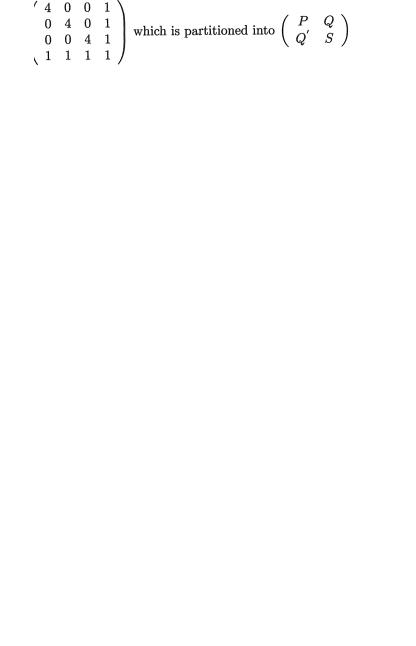
4. Functions of Random Variables and Sampling Distribution |
215 |
namely, N4( , Σ) with = 0 and
with the matrices and vectors P3×3 = 4I, Q’1×3 = (111) and S1×1 = 1. The matrix Σ is p.d. and it is easy to check that det(Σ) = 16.
Let us denote the matrices
Thus, applying (4.8.10), we have
and hence
In other words, in this particular situation, the pdf from (4.6.1) will reduce to
for (x1, x2, x3, x4) 4. Thus, in the Exercise 3.5.17, the given random vector X actually had this particular 4-dimensional normal distribution even though at that time we did not explicitly say so.
Sampling Distributions: The Bivariate Normal Case
For the moment, let us focus on the bivariate normal distribution. Suppose
that (X1, Y1), ..., (Xn, Yn) are iid  where –∞ < 1, 2 < ∞, 0 <
  < ∞ and –1 < ρ < 1, n ≥ 2. Let us denote
216 4. Functions of Random Variables and Sampling Distribution
Here, r is defined as the Pearson correlation coefficient or simply the sample correlation coefficient.
By separately using the marginal distributions of X1, ..., Xn and Y1, ..., Yn, we can right away claim the following sampling distributions:
The joint distribution of  is not very difficult to obtain by means of transformations. We leave this out as the Exercise 4.6.8.
Alternately, note, however, that any linear function of  and
and  is also a
linear function of the original iid random vectors (Xi, Yi), i = 1, ..., n. Then, by appealing to the Definition 4.6.1 of a multivariate normal distribution, we can immediately claim the following result:
How does one find ρ*? Invoking the bilinear property of covariance from Theorem 3.4.3, part (iii), one can express Cov  as
as
so that the population correlation coefficient between  and
and  is simplified
to n–1 ρσ1σ2 /  .
.
The distribution of the Pearson correlation coefficient
is quite complicated, particularly when ρ ≠ 0. Without explicitly writing down the pdf of r, it is still simple enough to see that the distribution of r can not
depend on the values of µ1,  and
and  . To check this claim, let us
denote Ui = (Xi – µ1)/σ1, Vi = (Yi – µ2)/σ2, and then observe that the random vectors (Ui, Vi), i = 1, ..., n, are distributed as iid N2(0, 0, 1, 1, ρ). But, r can be equivalently expressed in terms of the Ui’s and Vi’s as follows:
From (4.6.8), it is clear that the distribution of r depends only on ρ.
4. Functions of Random Variables and Sampling Distribution |
217 |
Francis Galton introduced a numerical measure, r, which he termed “reversion” in a lecture at the Royal Statistical Society on February 9, 1877 and later called “regression”. The term “cor-relation” or “correlation” probably appeared first in Galton’s paper to the Royal Statistical Society on December 5, 1888. At that time, “correlation” was defined in terms of deviations from the median instead of the mean. Karl Pearson gave the definition and calculation of correlation as in (4.6.7) in 1897. In 1898, Pearson and his collaborators discovered that the standard deviation of r happened to be  when n was large. “Student” derived the “probable error of a correlation coefficient” in 1908. Soper (1913) gave large sample approximations for the mean and variance of r which were better than those proposed earlier by Pearson. Refer to DasGupta (1980) for some of the historical details.
The unsolved problem of finding the exact pdf of r for normal variates came to R. A. Fisher’s attention via Soper’s 1913 paper. The pdf of r was published in the year 1915 by Fisher for all values of ρ (–1, 1). Fisher, at the age of 25, brilliantly exploited the n-dimensional geometry to come up with the solution, reputedly within one week. Fisher’s genius immediately came into limelight. Following the publication of Fisher’s results, however, Karl Pearson set up a major cooperative study of the correlation. One will notice that in the team formed for this cooperative project [Soper et al. (1917)] studying the distribution of the sample correlation coefficient, the young Fisher was not included. This happened in spite of the fact that Fisher was right there and he already earned quite some fame. Fisher felt hurt as he was left out of this project. One thing led to another. R. A. Fisher and Karl Pearson continued criticizing each other even more as each held on to his philosophical stand.
We will merely state the pdf of r when ρ = 0. This pdf is given by
where  for n ≥ 3. Using (4.6.9) and
some simple transformation techniques, one can easily derive the following result:
The verification of the claim in (4.6.10) is left as the Exercise 4.6.9. Fisher (1915) also gave the exact pdf of r in the form of an infinite power series for all values of ρ (–1, 0) (0, 1).

218 4. Functions of Random Variables and Sampling Distribution
Sampling Distributions : The Multivariate Normal Case
Now, we briefly touch upon some aspects of sampling distributions in the context of a multivariate normal population. Suppose that X1, ..., Xn are iid Np( , Σ) where p and Σ is a p × p p.d. matrix, n ≥ 2. Let us denote
Observe that  is a p-dimensional column vector whereas W is a p × p matrix, both functionally depending on the random samples X1, ..., Xn.
Theorem 4.6.1 Suppose that X1, ..., Xn are iid Np( , Σ) where p and Σ is a p × p p.d. matrix, n ≥ 2. Then, we have the following sampling distributions:
The part (i) in this theorem is easily proved by applying the Definition 4.6.1. Also, the part (ii) can be easily proved when p = 2. We leave their verifications out in the Exercise 4.6.10. Proofs of parts (ii)-(iv) in their fullest generality are, however, out of scope for this book. The readers, however, should exploit these results to avoid laborious calculations whenever possible.
4.6.2 The t Distribution
This distribution comes up frequently in the areas of multiple comparisons and selection and ranking. Let the random vector X, where X’ = (X1, ..., Xp), have a p-dimensional normal distribution with the mean vector 0 and the p × p dispersion matrix Σ. We assume that each diagonal entry in Σ is 1. That is, the random variables X1, ..., Xp have each been standardized. In other words, the (i, j)th entry in the matrix Σ corresponds to the population correlation coefficient ρij between the two variables Xi, Xj, 1 ≤ i ≠ j ≤ p. In this special situation, one also refers to Σ as a correlation matrix. Suppose that Y is a positive real valued random variable distributed as  . It is also assumed that Y and (X1, ..., Xp) are independent. Let us denote p new random variables
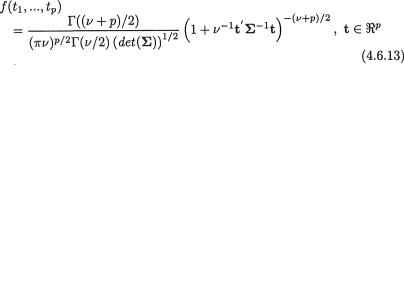
4. Functions of Random Variables and Sampling Distribution |
219 |
The marginal distribution of each Ti has the Student’s t distribution with ν degrees of freedom. This follows from the definition of the Student’s t random variable. Jointly, however, (T1, ..., Tp) is said to have the p-dimensional t distribution which depends on the correlation matrix Σ, denoted by Mtp(ν, Σ). One may refer to Johnson and Kotz (1972, p. 134). If we assume that Σ–1 exists, then the joint pdf of T1, ..., Tp, distributed as Mtp(ν, Σ), is given by
with t’ = (t1, ..., tp). The derivation of this joint pdf is left as the Exercise 4.6.11.
Fundamental works in this area include references to Cornish (1954, 1962), Dunnett (1955), and Dunnett and Sobel (1954, 1955), among others. One may also refer to Johnson and Kotz (1972) and Tong (1990) to find other sources.
Example 4.6.6 Suppose that Ui1, ..., Uini are iid N(µi, σ2), i = 1, 2, 3 as in the setup of a one-way analysis of variance. Let the three treatments be inde-
pendent too. From the ith treatment, we obtain the sample mean  and the sample variance
  . Since the population variances are all equal to σ2, we obtain the pooled sample variance
Let  . Then, (X1, X2) is distributed as N2(0, Σ) with
 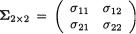 where σ11 =
σ 22 = 1 and σ12 = σ21 =  . Also,
 is distributed as a Chi-square random variable with the degree of freedom ν = n1 + n2 + n3 – 3. Next, the random variable Y and the random vector (X1, X2) are independently distributed. Thus, with
  , i = 1, 2, the corresponding random vector (T1, T2) is distributed as Mt2(ν, Σ). !
4.6.3 The F Distribution
This distribution also arises frequently in the areas of analysis of variance, multiple comparisons, and selection and ranking. Suppose that we have

220 4. Functions of Random Variables and Sampling Distribution
independent random variables X0, X1, ..., Xp where Xi is distributed as  , i = 0, 1, ..., p. This is often the situation in the case of analysis of variance, where these X’s customarily stand for the sums of squares due to
the error and treatments. We denote the new random variables
The marginal distribution of the random variable Ui is F νi, ν0. This follows from the definition of a F random variable. Jointly, however, (U1, ..., Up) is said to have the p-dimensional F distribution, denoted by MFp(ν0, ν1, ..., νp). One may refer to Johnson and Kotz (1972, p. 240). The joint pdf of U1, ..., Up, is distributed as MFp(ν0, ν1, ..., νp), is given by
with u’ = (u1, ..., up) and  . The derivation of this joint pdf is left as the Exercise 4.6.13.
Fundamental works in this area include references to Finney (1941) and Kimbal (1951), among others. One may also refer to Johnson and Kotz (1972) and Tong (1990) to find other sources.
4.7Importance of Independence in Sampling Distributions
In the reproductive property of the normal distributions and Chi-square distributions (Theorem 4.3.2, parts (i) and (iii)) or in the definitions of the Student’s t and F distributions, we assumed independence among various random variables. Now, we address the following important question. If those independence assumptions are violated, would one have similar standard distributions in the end? In general, the answer is “no” in many circumstances. In this section, some of the ramifications are discussed in a very simple way.
4.7.1 Reproductivity of Normal Distributions
In the Theorem 4.3.2, part (i), we learned that independent normal variables add up to another normal random variable. According to the Definition 4.6.1, as long as (X1, ..., Xn) is distributed as the n-dimensional normal Nn, this reproductive property continues to hold. But, as soon as we stray
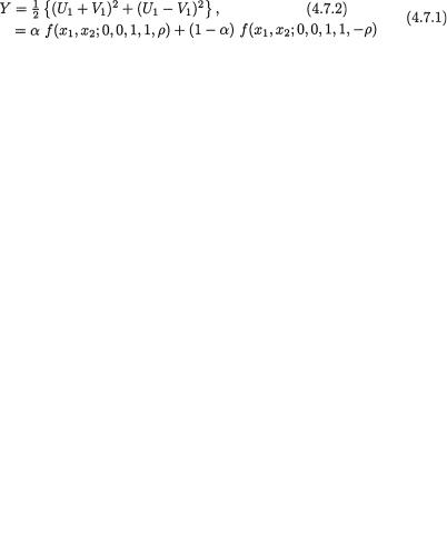
4. Functions of Random Variables and Sampling Distribution |
221 |
away from the structure of the multivariate normality for (X1, ..., Xn), the marginals of X1, ..., Xn can each be normal in a particular case, but their sum need not be distributed as a normal variable. We recall an earlier example.
Example 4.7.1 (Example 3.6.3 Continued) Let us rewrite the bivariate normal pdf given in (3.6.1) as  . Next, consider any arbitrary 0 < α, ρ < 1 and fix them. We recall that we had
for –∞ < x1, x2 ∞. Here, (X1, X2) has a bivariate non-normal distribution, but marginally both X1, X2 have the standard normal distribution. However one can show that X1 + X2 is not a univariate normal variable. These claims are left as the Exercises 4.7.1.-4.7.2. !
4.7.2 Reproductivity of Chi-square Distributions
Suppose that X1 and X2 are independent random variables which are respectively distributed as  and
and  . From the Theorem 4.3.2, part (iii), we can then claim that X1 + X2 will be distributed as
  . But, will the same conclusion necessarily hold if X1 and X2 are respectively distributed as
  and
and  , but X1 and X2 are dependent? The following simple example shows that when X1 and X2 are dependent, but X1 and X2 are both Chi-squares, then X1 + X2 need not be Chi-square.
Example 4.7.2 Suppose that (U1, V1) is distributed as N2(0, 0, 1, 1, ρ). We assume that –1 < ρ < 1. Let  and thus the marginal distributions of X1, X2 are both
  . Let us investigate the distribution of Y = X1 + X2. Observe that
where the joint distribution of (U1 + V1, U1 – V1) is actually N2, because any linear function of U1 + V1, U1 – V1 is ultimately a linear function of U1 and V1, and is thus univariate normal. This follows (Definition 4.6.1) from the fact that (U1, V1) is assumed N2. Now, we can write
and hence from our earlier discussions (Theorem 3.7.1), it follows that U1 + V1 and U1 – V1 are independent random variables. Also, U1 + V1 and U1 – V1 are respectively distributed as N (0, 2(1 + ρ)) and N (0, 2(1 – ρ)).

222 4. Functions of Random Variables and Sampling Distribution
Thus, with 0 < t < min {(2(1 + ρ))–1, (2(1 – ρ))–1}, the mgf MY(t) of Y is given by
Hence, we can express MY(t) as
which will coincide with (1 – 2t)–1, the mgf of  , if and only if ρ = 0. We have shown that Y is distributed as
  if and only if ρ = 0, that is if and only if X1, X2 are independent. !
We have not said anything yet about the difference of random variables which are individually distributed as Chi-squares.
The difference of two Chi-square random variables may or may not be another Chi-square variable. See the Example 4.7.3.
Example 4.7.3 Suppose that we have X1, X2, X3, X4 which are iid N(0, 1).
Let us denote |
. Since |
s are iid |
i |
= 1, 2, 3, 4, by the reproductive property of Chi-square distributions we claim that U1 is distributed as  Obviously, U2 is distributed as
  At the same time, we have
  which is distributed as
  Here, the difference of two Chi-square random variables is distributed as another Chisquare variable. Next, let us we denote
  which is distributed as
  But,
But,  and this random variable cannot have a Chi-square distribution. We can give a compelling reason to support this conclusion. We note that U1 – U3 can take negative values with positive probabil-
ity. In order to validate this claim, we use the pdf of F2,1 and express as
which simplifies to 1 – 2–1/2 ≈ .29289. !
Let X1, ..., Xn be iid N(µ, µ2) and S2 be the sample variance. Then, (n – 1)S2/σ2 is distributed as Chi-square. Is it possible that (n – 1)S2/σ2 is a Chi-square random variable without the assumed normality of the X’s? See the Exercise 4.7.4.
4. Functions of Random Variables and Sampling Distribution |
223 |
4.7.3 The Student’s t Distribution
In the Definition 4.5.1, we introduced the Student’s t distribution. In defining W, the Student’s t variable, how crucial was it for the standard normal variable X and the Chi-square variable Y to be independent? The answer is: independence between the numerator and denominator was indeed very crucial. We elaborate this with the help of two examples.
Example 4.7.4 Suppose that Z stands for a standard normal variable and we let X = Z, Y = Z2. Clearly, X is N(0, 1) and Y is  but they are dependent random variables. Along the line of construction of the random variable W, let us write
  and it is clear that W can take only two
values, namely –1 and 1, each with probability 1/2 since P(X > 0) = P(X ≤ 0) = 1/2. That is, W is a Bernoulli variable instead of being a t variable. Here, W
has a discrete distribution! !
Example 4.7.5 Let X1, X2 be independent, X1 being N(0, 1) and X2 being
. Define X = X1,  , and obviously we have X2 < Y w.p. 1, so that X and Y are indeed dependent random variables. Also by choice, X is N(0, 1) and Y is
  . Now, consider the Definition 4.5.1 again and write
so that we have | W |≤ (n + 1)1/2. A random variable W with such a restricted domain space can not be distributed as the Student’s t variable. The domain space of the t variable must be the real line, . Note, however, that the random variable W in (4.7.4) has a continuous distribution unlike the scenario in
the previous Example 4.7.4. !
4.7.4 The F Distribution
In the Definition 4.5.2, the construction of the F random variable was explained. The question is whether the independence of the two Chi-squares, namely X and Y, is essential in that definition. The answer is “yes” as the following example shows.
Example 4.7.6 Let U1, U2 be independent, U1 be  and U2 be
  . Define X = U1, Y = U1 + U2, and we note that Y > X w.p.1. Hence, obviously X,Y are dependent random variables. Also, X is
  and Y is
  . Now, we look at the Definition 4.5.2 and express U as
so that we have 0 < U < (m + n)/m. A random variable U with such a restricted domain space cannot have F distribution. The domain space
224 4. Functions of Random Variables and Sampling Distribution
of F variable must be +. Note, however, that the random variable U in (4.7.5) has a continuous distribution.
4.8 Selected Review in Matrices and Vectors
We briefly summarize some useful notions involving matrices and vectors made up of real numbers alone. Suppose that Am×n is such a matrix having m rows and n columns. Sometimes, we rewrite A as (a1, ..., an) where ai stands for the ith column vector of A, i = 1, ..., n.
The transpose of A, denoted by A’, stands for the matrix whose rows consist of the columns a1, ..., an of A. In other words, in the matrix A’, the row vectors are respectively a1, ..., an. When m = n, we say that A is a square matrix.
Each entry in a matrix is assumed to be a real number.
The determinant of a square matrix An×n is denoted by det(A). If we have two square matrices An×n and Bn×n, then one has
The rank of a matrix Am×n = (a1, ..., an), denoted by R(A), stands for the maximum number of linearly independent vectors among a1, ..., an. It can be
shown that
A square matrix An×n = (a1, ..., an) is called non-singular or full rank if and only if R(A) = n, that is all its column vectors a1, ..., an are linearly
independent. In other words, An×n is non-singular or full rank if and only if the column vectors a1, ..., an form a minimal generator of n.
A square matrix Bn×n is called an inverse of An×n if and only if AB = BA = In×n, the identity matrix. The inverse matrix of An×n, if it exists, is unique and it is customarily denoted by A–1. It may be worthwhile to recall the following
result.
For a matrix An×n: A–1 exists R(A) = n det(A) ≠ 0.
For a 2 × 2 matrix  , one has det(A) = a11a22 – a12a21.
Let us suppose that a11a22 ≠ a12a21, that is det(A) ≠ 0. In this situation, the inverse matrix can be easily found. One has:
4. Functions of Random Variables and Sampling Distribution |
225 |
A square matrix An×n is called orthogonal if and only if A’, the transpose of
A, is the inverse of A. If An×n is orthogonal then it can be checked that det(A) = ±1.
A square matrix A = (aij)n×n is called symmetric if and only if A’ = A, that is aij = aji, 1 ≤ i ≠ j ≤ n.
Let A = (aij, i,j = 1, ..., n, be a n×n matrix. Denote the l×l sub-matrix Bl = (apq), p, q = 1, ..., l,l = 1, ..., n. The lth principal minor is defined as the
det(Bl), l = 1, ..., n.
For a symmetric matrix An×n, an expression such as x’ Ax with x n is customarily called a quadratic form.
A symmetric matrix An×n is called positive semi definite (p.s.d.) if (a) the quadratic form x’ Ax ≥ 0 for all x k, and (b) the quadratic form x’ Ax =0 for some non-zero x n.
A symmetric matrix An×n is called positive definite (p.d.) if (a) the quadratic form x’ Ax ≥ 0 for all x n, and (b) the quadratic form x’ Ax =0 if and only if x = 0.
A symmetric matrix An×n is called negative definite (n.d.) if (a) the quadratic form x’ Ax ≤0 for all x n, and (b) the quadratic form x’ Ax =0 if and only if x = 0. In other words, a symmetric matrix An×n is n.d. if and only if – A is positive definite.
Let us now look at some partitioned matrices A, B where
where m, n, u, v, w, t, c, d are all positive integers such that u + w = m, u + t = n and c + d = q. Then, one has
226 4. Functions of Random Variables and Sampling Distribution
Again, let us consider a partitioned matrix A from (4.8.7) where Pu×u and Sw×w are square matrices where u + w = n. Then, one has
Let us reconsider the partitioned matrix An×n which was used in (4.8.9). Then, we can write
Next, we summarize an important tool which helps us to find the maximum or minimum of a real valued function of two variables. The result follows:
Suppose that f(x) is a real valued function of a two-dimensional variable x = (x1, x2) (a1, b1) × (a2, b2) 2, having continuous second-order partial
derivatives  and
and 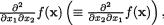 everywhere
in an open rectangle (a1, b1) × (a2, b2). Suppose also that for some point ξ = (ξ1, ξ2) (a1, b1) × (a2, b2), one has
Now, let us denote the matrix of the second-order partial derivatives
Then,
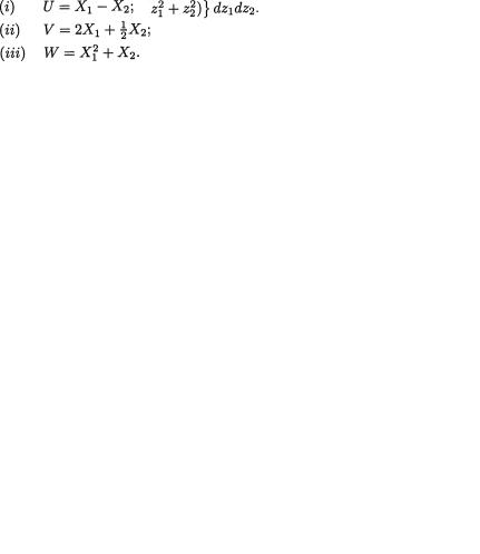
4. Functions of Random Variables and Sampling Distribution |
227 |
4.9Exercises and Complements
4.1.1(Example 4.1.1 Continued) Suppose that Z1, Z2 are iid standard
normal variables. Evaluate  with some fixed but arbitrary b >
0. {Hint: Express |
the required probability as the double integral, |
|
. Use the substitutions from (4.1.1) |
to rewrite this as |
which will change to |
|
. This last integral can then be re- |
placed by |
|
Also, look at the Exercise 4.5.7.}
4.2.1 (Example 4.2.1 Continued) Consider the two random variables X1, X2 from the Example 4.2.1. Find the pmf’s of the following random variables which are functions of X1, X2.
4.2.2 Let X1, X2 be iid Poisson(λ), λ > 0. Derive the distribution of the random variable U = X1 + X2. Then, use mathematical induction to show that  has the Poisson(nλ) distribution if X1, ..., Xn are iid Poisson(λ). Next, evaluate P(X1 – X2 = v) explicitly when v = 0, 1, 2, 3. Proceeding this way, is it possible to write down the pmf of the random variable V = X1 – X2? {Hint: In the first part, follow along the Examples 4.2.2-4.2.3.}
4.2.3 In a Bernoulli experiment, suppose that X1 = number of trials needed to observe the first success, and X2 = number of trials needed since the first success to observe the second success, where the trials are assumed independent having the common success probability p, 0 < p < 1. That is, X1, X2 are assumed iid having the Geometric(p) distribution defined earlier in (1.7.7). First, find the distribution of the random variable U = X1 + X2. Next, with k such iid random variables X1, ..., Xk, derive the pmf of the random variable
. The distribution of U is called Negative Binomial with parameters (k, p). A different parameterization was given in (1.7.9).
4.2.4 Let the pdf of X be  with β > 0. Find the pdf’s of the following random variables which are functions of X.
(i)U = X2;
(ii)V = X3.
2284. Functions of Random Variables and Sampling Distribution
4.2.5In general, suppose that X1, ..., Xn are iid continuous random variables with the common pdf and df respectively given by f(x) and F(x). Derive the joint pdf of the ith
order statistic Yi = Xn:i and the jth order statistic Yj = Xn:j, 1 ≤ i < j ≤ n by solving the following parts in the order
that
(i)(U1, U2, U3) is distributed as multinomial with k = 3, p1 = F(u1), p2 = F(u2) – F(u1), and p3 = 1 – p1 – p2 = 1 – F(u2);
(ii)P{Yi ≤ u1 ∩ Yj ≤ u2} = P{U1 ≥ i ∩ (U1 + U2) ≥ j};
(iii)  U2 = l} + P{U ≥ j};
(iv)the expression in part (iii) can be rewritten as
(v)the joint pdf of Yi, Yj, denoted by f(yi, yj), can be directly obtained by evaluating 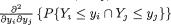 first,
and then simplifying it.
4.2.6 Verify (4.2.7). {Hint: Use the Exercise 4.2.5.}
4.2.7 Suppose that X1, ..., Xn are iid uniform random variables on the
interval (0, θ), θ . Denote the ith order statistic Yi = Xn:i where Xn:1 = Xn:2
≤ ... ≤ Xn:n. Define U = Yn – Y1, V = 1/2(Yn + Y1) where U and V are respectively referred to as the range and midrange for the data X1, ..., Xn.
This exercise shows how to derive the pdf of the range, U.
(i)Show that the joint pdf of Y1 and Yn is given by h(y1, yn) = n(n – 1)θ–n (yn – y1)n–2 I(0 < y1 < yn < θ). {Hint: Refer to the equation (4.2.7).};
(ii)Transform (Y1, Yn) to (U, V) where U = Yn – Y1, V = 1/2(Yn + Y1). Show that the joint pdf of (U, V) is given by g(u, v) = n(n – 1) θ–n un–2 when 0 < u < θ, 1/2u < v < θ – 1/2u, and zero otherwise;
(iii)Show that the pdf of U is given by g1(u) = n(n – 1)θ–n × (θ – u) un–2 I(0 < u < θ). {Hint: g1(u) =  ,
,
for 0 < u < θ.};
(iv)When θ = 1, does the pdf of the range, U, derived in part (iii) correspond to that of one of the standard random variables from
the Section 1.7?
4.2.8 Suppose that X1, ..., Xn are iid uniform random variables on the interval (θ, θ + 1), θ . Denote the ith order statistic Yi = Xn:i where
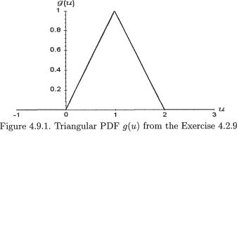
4. Functions of Random Variables and Sampling Distribution |
229 |
Xn:1 ≤ Xn:2 ≤ ... ≤ Xn:n. Define U = Yn – Y1, V = 1/2(Yn + Y1) where recall that U and V are respectively referred to as the range and midrange for the data
X1, ..., Xn. This exercise shows how to derive the pdf of the range, U.
(i)Show that the joint pdf of Y1 and Yn is given by h(y1, yn) = n(n – 1)(yn – y1)n–2 I(θ < y1 < yn < θ + 1). {Hint: Refer to the equation (4.2.7).};
(ii)Transform (Y1, Yn) to (U, V) where U = Yn – Y1, V = 1/2(Yn + Y1). Show that the joint pdf of (U, V) is given by g(u, v) = n(n
– 1)un–2 when 0 < u < 1, θ + 1/2u < v < θ + 1 – 1/2u, and zero otherwise;
(iii)Show that the pdf of U is given by g1(u) = n(n – 1)×(1 – u) un–2 I(0 < u < 1). {Hint:g1(u)= ,for 0<u< 1.};
(iv)Does the pdf of the range, U, derived in part (iii) correspond to that of one of the standard random variables from the Section 1.7?
4.2.9 (Triangular Distribution) Suppose that X1 and X2 are independent random variables, distributed uniformly on the interval (0, 1) with the respec-
tive pdf’s f1(x1) = I(0 < x1 < 1) and f2(x2) = I(0 < x2 < 1). Show that the pdf of U = X1 + X2 is given by
The random variable U is said to follow the triangular distribution. Look at the plot of g(u) in the Figure 4.9.1. {Hint: It is obvious that the pdf g(u) of
230 4. Functions of Random Variables and Sampling Distribution
U will be zero when u ≤ 0 or u ≥ 2, but it will be positive when 0 < u < 2. Thus, using the convolution result, for 0 < u < 1, we can write the df of U as
 . Hence, for 0 < u < 1 we have
  . On the other hand, for 1 ≤ u < 2, we can write the df of U as
so that 
4.2.10Suppose that X1 and X2 are independent random variables, distributed uniformly on the intervals (0, 1) and (0, 2) with the respective pdf’s
f1(x1) = I(0 < x1 < 1) and f2(x2) = 1/2I(0 < x2 < 2). Use the convolution result to derive the form of the pdf g(u) of U = X1 + 1/2X2 with 0 < u < 2.
4.2.11(Example 4.2.10 Continued) Let U, V be iid N(µ, σ2). Find the pdf of W = U + V by the convolution approach. Repeat the exercise for the random variable T = U – V.
4.2.12(Example 4.2.11 Continued) Provide all the intermediate steps in the Example 4.2.11.
4.2.13Prove a version of the Theorem 4.2.1 for the product, V = X1X2, of two independent random variables X1 and X2 with their respective pdf’s given by f1(x1) and f2(x2). Show that the pdf of V is given by h(v) =
for v . Show that h(v) can be equivalently
written as  . {Caution: Assume that V can not take the value zero.}
4.2.14 Suppose that X1, X2, X3 are iid uniform random variables on the interval (0, 1).
(i)Find the joint pdf of X3:1, X3:2, X3:3;
(ii)Derive the pdf of the median, X3:2;
(iii)Derive the pdf of the range, X3:3 – X3:1. {Hint: Use the Exercise 4.2.7}
4.2.15 Suppose that X1, ..., Xn are iid N(0, 1). Let us denote Yi = 4Φ(Xi) where  .
.
(i)Find the pdf of the random variable 
(ii)Evaluate E[U] and V[U];
(iii)Find the marginal pdf’s of Yn:1, Yn:n and Yn:n – Yn:1.
4.2.16 Suppose that X1 is uniform on the interval (0, 2), X2 has its pdf 1/ 2xI(0 < x < 2), and X3 has its pdf 3/8x2I(0 < x < 2). Suppose also that X1, X2, X3 are independent. Derive the marginal pdf’s of X3:1 and X3:3. {Hint: Follow along the Example 4.2.8.}
4. Functions of Random Variables and Sampling Distribution |
231 |
4.2.17 Suppose that Z is the standard normal random variable. Denote X = max{|Z|, 1/|Z|}.
(i)Find the expression of P{X ≤ x} for x ≥ 1. Observe that P{X ≤ x} = 0 for x < 1;
(ii)Use part (i) to show that the pdf of X is given by f(x) = 2{φ(x) + x–2φ(x–1)}I(x ≥ 1).
{Hint: For x = 1, one can write P{X ≤ x} = P{x–1 ≤ |Z|≤ x} = 2P{x–1 ≤ Z = x} = 2{Φ(x) – Φ(x–1)}. This is part (i). Differentiating this expression with respect to x will lead to part (ii).}
4.2.18 (Exercise 4.2.9 Continued) Suppose that X1, X2 and X3 are independent random variables, distributed uniformly on the interval (0, 1) with the
respective pdf’s f1(x1) = I(0 < x1 < 1), f2(x2) = I(0 < x2 < 1) and f3(x3) = I(0 < x3 < 1). Use the convolution result to derive the form of the pdf h(v) of V =
X1 + X2 + X3 with 0 < v < 3. {Hint: Note that V = U + X3 where U = X1 + X2 and its pdf g(u) was derived in the Exercise 4.2.9 for 0 < u < 2. Now, use the
convolution result again.}
4.2.19 (Example 4.2.9 Continued) Suppose that X1, X2 and X3 are independent random variables, distributed exponentially with the respective pdf’s
f1(x1) = e–x1I(x1 +), f2(x2) = e–x2I(x2 +) and f3(x3) = e–x3I(x3 +). Use the convolution result to show that the pdf h(v) of V = X1 + X2 + X3 with v
+ matches with that of the Gamma(3, 1) distribution. {Hint: Note that V = U + X3 where U = X1 + X2 and its pdf g(u) was derived in the Example 4.2.9 for u +. Now, use the convolution result again.}
4.2.20 Suppose that X1, ..., Xn are iid Uniform(0, 1) random variables where n = 2m + 1 for some positive integer m. Consider the sample median, that is U = Xn:m+1 which is the order statistic in the middle.
(i)Show that the pdf of U is given by g(u) = cum(1 – u)m × I(0 < u < 1) where c = (2m + 1)!/(m!)2. Is this one of the standard distributions listed in the Section 1.7?
(ii)Show that E(U) = 1/2 and  .
.
4.3.1Suppose that X1, ..., Xn are iid Poisson(λ). Use the mgf technique to show that  has the Poisson(nλ) distribution. {Hint: Follow along the Examples 4.3.1-4.3.2.}
4.3.2Suppose that X1, ..., Xk are iid Geometric(p), 0 < p < 1. Find the
distribution of  . The distribution of U is called Negative Binomial with parameters (k, p). A different parameterization was given in (1.7.9).
4.3.3Complete the arguments in the Example 4.3.5.
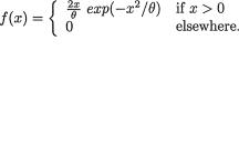
2324. Functions of Random Variables and Sampling Distribution
4.3.4Consider the two related questions.
(i)Suppose that a random variable U has its pdf given by g(u) =
1-σe–|u|/σI(–∞ < u < ∞). First show that the mgf of U is given by
2
(1– σ2t2)–1 for |t|< σ–1, with 0 < σ < ∞;
(ii)Next, suppose that X1, X2 are iid with the common pdf f(x) ,  with β > 0. Using part (i), derive the pdf
of V = X1 – X2.
4.3.5 Let Y1, Y2 be iid N (0, 4). Use the mgf technique to derive the distribution of  . Then, obtain the exact algebraic expressions for
(i)P(U > 1);
(ii)P(1 < U < 2);
(iii)P(| U – 2 |≥ 2.3).
4.3.6Suppose that Z is the standard normal variable. Derive the expression of E[exp(tZ2)] directly by integration. Hence, obtain the distribution of
Z2.
4.3.7(Exercise 4.3.6 Continued) Suppose that the random variable X is distributed as N(µ, σ2), µ , σ +. Obtain the expression of the mgf of the random variable X2, that is E[exp(tX2)].
4.3.8Prove the Theorem 4.3.2.
4.3.9Suppose that U1, ..., Un are iid random variables with the common pdf given by  . Then, use the
part (ii) or (iii) from the Theorem 4.3.2 to obtain the distribution of the random variable  .
.
4.4.1 Let X be a random variable with the pdf
Find the marginal pdf’s of U, V, and W defined as follows:
(i)U = 2X – 1; (ii) V = X2; (iii) 
4.4.2Suppose that a random variable X has the Raleigh density given by
Derive the pdf of U = X2.
4.4.3 (Example 4.4.3 Continued) Suppose that Z has the standard normal distribution. Let us denote Y = |Z|. Find the pdf of Y. {Caution: The
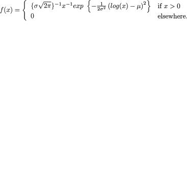
4. Functions of Random Variables and Sampling Distribution |
233 |
transformation from Z to Y is not one-to-one. Follow along the Example 4.4.3.}
4.4.4(Example 4.4.3 Continued) Suppose that Z has the standard normal distribution. Let us denote Y = |Z|3. Find the pdf of Y. {Caution: The transformation from Z to Y is not one-to-one. Follow along the Example 4.4.3.}
4.4.5(Example 4.4.4 Continued) Suppose that X has the pdf f(x) = 1/ 2exp{– |x|}I(x ). Obtain the pdf of Y = |X|3. {Caution: The transformation from X to Y is not one-to-one. Follow along the Example 4.4.4.}
4.4.6(Example 4.4.7 Continued) Verify all the details.
4.4.7(Example 4.4.8 Continued) Verify all the details.
4.4.8Suppose that X1, ..., Xn are iid Uniform(0, 1). Let us define Yi = Xn:i/ Xn:i–1, i = 1, ..., n with Xn:0 = 1. Find the joint distribution of Y2, ..., Yn. {Hint: First, consider taking log and then use the results from Examples 4.4.2 and
4.4.10.}
4.4.9 (Example 4.4.9 Continued) Suppose that X1, ..., Xn are iid N(µ, σ2) with n ≥ 2. Use the Helmert variables Y1, ..., Yn from the Example 4.4.9 to show that ( – 1)2 and S + S2/3 are independently distributed.
4.4.10 Suppose that (U, V) has the following joint pdf:
where θ > 0. Define X = UV and Y = U/V.
(i) Find the joint pdf of (X, Y); (ii) Find the marginal pdf’s of X, Y;
(iii) Find the conditional pdf of Y given X = x.
4.4.11 Let X1, X2 be iid having the Gamma(α, β) distribution with α > 0, β > 0. Let us denote U = X1 + X2, V = X2/X1. Find the marginal distributions of
U, V.
4.4.12 Let X1, X2 be iid N(µ, σ2). Define U = X1 + X2, V = X1 – X2.
(i)Find the joint pdf of (U, V);
(ii)Evaluate the correlation coefficient between U and V;
(iii)Evaluate the following: E{(X1 – X2)2 &pipe; X1 + X2 = x}; E{(X1 + X2)2 | X1 = X2}; V{(X1 – X2)2 | X1 + X2 = x}.
4.4.13Suppose that X has the following pdf with –∞ < µ < ∞, 0 < µ < ∞:

234 4. Functions of Random Variables and Sampling Distribution
One will recall from (1.7.27) that this pdf is known as the lognormal density and the corresponding X is called a lognormal random variable. Suppose that X1, X2 are iid having the common pdf f(x). Let r and s be arbitrary, but fixed
real numbers. Then, find the pdf of the random variable |
{Hint: Does |
taking log help?}
4.4.14 Suppose that X1, X2, X3 are iid Gamma(α, β), α > 0, β > 0. Define
U1 = X1 + X2 + X3, U2 = X2/(X1 + X2), and U3 = X3/(X1 + X2 + X3). Solve the following problems.
(i)Show that one can express x1 = u1(1 – u2)(1 – u3), x2 = u1u2(1 – u3), x3. Is this transformation one-to-one?
(ii)Determine the matrix J from (4.4.3) and show that | det(J) | =  ;
;
(iii)Start out with the joint pdf of X1, X2, X3. Use the transformation (x1, x2, x3) → (u1, u2, u3) to obtain the joint pdf of U1, U2, U3;
(iv)Argue that U1, U2, U3 are distributed independently. Show that (a) U1 is distributed as Gamma(3α, β), (b) U2 is distributed as Beta(α, α), and (c) U3 is distributed as Beta(α, 2α). In this part, recall the beta function and the Beta pdf from (1.6.25)- (1.6.26) and (1.7.35) respectively.
4.4.15 Suppose that X1, X2, X3, X4 are iid Gamma(α, β), α > 0, β > 0.
Define U1 = X1 + X2 + X3 + X4, U2 = X2/(X1 + X2), U3 = X3/(X1 + X2 + X3), and U4 = X4/(X1 + X2 + X3 + X4). Solve the following problems.
(i)Show that one can express x1 = u1(1 – u2)(1 – u3)(1 – u4), x2 = u1u2(1 – u3)(1 – u4), x3 = u1u3(1 – u4), x4 = u1u4. Is this transfor mation one-to-one?
(ii)Determine the matrix J from (4.4.3) and show that | det(J) | = u1(1 – u2)(1 – u3)(1 – u4);
(iii)Start out with the joint pdf of X1, X2, X3, X4. Use the transforma tion (x1, x2, x3, x4) →u1, u2, u3, u4) to obtain the joint pdf of U1,
U2, U3, U4;
(iv)Argue that U1, U2, U3, U4 are distributed independently Show that (a) U1 is distributed as Gamma(4α, β), (b) U2 is distributed as Beta(α, α), (c) U3 is distributed as Beta(α, 2α), and (d) U4 is Beta(α, 3α). Recall the beta function and Beta pdf from (1.6.25)- (1.6.26) and (1.7.35) respectively.
4.4.16(Example 4.4.13 Continued) Provide all the details in the Example
4.4.13.
4.4.17(Example 4.4.14 Continued) Provide all the details in the Example
4.4.14.
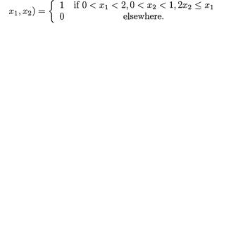
4. Functions of Random Variables and Sampling Distribution |
235 |
4.4.18 (Example 4.4.16 Continued) Suppose that (X1, X2) is distributed as N2(0, 0, σ2, σ2, ρ) with 0 < σ < ∞, –1 < ρ < 1. Define U = X1/X2 and V = X1.
(i) Find the joint pdf of U and V;
(ii) In part (i), integrate out V and derive the marginal pdf of U;
(iii) When ρ = 0, the pdf in part (ii) coincides with the standard Cauchy pdf, namely, π–1(1 + u2)–1 for –∞ < u < ∞
(iv) When ρ ≠ 0, the pdf in part (ii) coincides with the Cauchy pdf with appropriate location and scale depending on ρ.
4.4.19 Suppose that (X1, X2) has the following joint pdf:
Find the pdf of U = X1 – X2. {Hint: Use the transformation u = x1 – x2 and v = x1.}
4.4.20 Suppose that (X1, X2) has the following joint pdf:
Show that the pdf of  is given by
4.4.21 Suppose that (X1, X2) has the following joint pdf:
Let U = X1 + X2 and V = X1X2.
(i)Show that the pdf of U is a(u)
(ii)Show that the pdf of V is b(v) 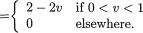
4.4.22Suppose that X1, X2 are iid random variables. We are told that X1 + X2 and X1 – X2 are independently distributed. Show that the common pdf of X1, X2 must be same as the normal density. {Hint: Can the Remark 4.4.4 be used to solve this problem?}
4.4.23Suppose that X1, X2, X3 are three iid random variables. We are also told that X1 + X2 + X3 and (X1 – X2, X1 – X3) are independently
236 4. Functions of Random Variables and Sampling Distribution
distributed. Show that the common pdf of X1, X2, X3 must be the normal pdf. {Hint: Can the Remark 4.4.4 be used to solve this problem?}
4.5.1In the Theorem 4.5.1, provide all the details in the derivation of the pdf of tí, the Student’s t with ν degrees of freedom.
4.5.2Consider the pdf h(w) of tí, the Student’s t with ν degrees of free-
dom, for w . In the case ν = 1, show that h(w) reduces to |
the |
Cauchy density. |
|
4.5.3Generalize the result given in the Example 4.5.2 in the case of the k- sample problem with k(≥ 3).
4.5.4With n(≥ 4) iid random variables from N(0, σ2), consider the Helmert variables Y1, ..., Y4 from Example 4.4.9. Hence, obtain the distribution
of |
and that of W2? |
4.5.5 Suppose that X1, ..., Xn are iid random variables having a common pdf given by f(x) = σ–1 exp{–(x – )/σ}I(x > ) for – ∞ < µ < ∞, 0 < σ < ∞. Here, is the location parameter and ó is the scale parameter. Consider (4.4.18) and let U = n(Xn:1 – µ) / σ, V = 2T / σ.
(i)Find the pdf of U and E(Ur) for all fixed numbers r > 0;
(ii)Evaluate E(Vr) for all fixed real numbers r;
(iii)What is the distribution of W = σU ÷ [T/(n – 1)]?
{Caution: In parts (i)-(ii), watch for the condition on n as needed.}
4.5.6 Suppose that X1, ..., Xn are iid N(µ, σ2). Recall the Helmert variables Y1, ..., Yn from the Example 4.4.9.
(i) Find the pdf of Yi/Yj for i ≠ j = 2, ..., n; (ii) Find the pdf of Yi/ |Yj| for i ≠ j = 2, ..., n; (iii) Find the pdf of Yi2 / Yj2 for i ≠ j = 2, ..., n;
(iv) Find the pdf of Yi2 / T where 
(v) Find the pdf of  /U where for i ≠ j = 2, ..., n.
{Hint: Recall the distributional properties of the Helmert variables.}
4.5.7 (Exercise 4.1.1 Continued) Let Z1, Z2 be iid standard normal. From the Exercise 4.5.2, note that the random variable Z1/Z2, denoted by X, has the Cauchy pdf given in (1.7.31). Use this sampling distribution to evaluate  where b(> 0) is fixed but arbitrary. {Hint: Express the re-
quired probability as  and then integrate the Cauchy pdf
within the appropriate interval. Does this match with the answer given for the Exercise 4.1.1?}
4.5.8 (Exercise 4.5.7 Continued) Let Z1, Z2 be iid standard normal. Evaluate where c is a fixed but arbitrary real number.
4. Functions of Random Variables and Sampling Distribution |
237 |
4.5.9(Exercise 4.5.8 Continued) Let Z1, Z2 be iid standard normal. Evaluate  where 0 < c < 1 is a fixed but arbitrary number.
4.5.10Verify the expression of the variance of W, which is distributed as tí, given in (4.5.4).
4.5.11Verify the expression of the mean and variance of U, which is distributed as Fí1,í2, given in (4.5.11)-(4.5.12).
4.6.1(Example 4.6.1 Continued) Use transformations directly to show
that (X1,  ) is distributed as
  when X1, ..., Xn are iid N(µ, σ2).
4.6.2(Example 4.6.2 Continued) Use transformations directly to find the
bivariate normal distribution of (aX1 + bX2,  ) when X1, ..., Xn are iid N(µ σ2). Here, a and b are fixed non-zero real numbers.
4.6.3Show that the bivariate normal density from (3.6.1) can be expressed in the form given by (4.6.1).
4.6.4Verify the properties given in (4.6.2)-(4.6.3) for the multivariate normal distribution.
4.6.5Let X1, ..., Xn be iid N(µ, σ2). Then, find the joint distributions of
(i)Y2, ..., Yn where Yi = Xi – X1, i = 2, ..., n;
(ii)U2, ..., Un where Ui = Xi – Xi–1, i = 2, ..., n.
{Hint: Use the Definition 4.6.1 for the multivariate normality.}
4.6.6(Exercise 4.6.5 Continued) Solve the Exercise 4.6.5 by using direct transformation techniques.
4.6.7Suppose that X1, ..., Xn are iid N(µ, σ2), n ≥ 2. Use the variables U1,
..., Un where 
(i)Show that U = (U1, ..., Un) has the n-dimensional normal distri bution;
(ii)Show that U1 and (U2, ..., Un) are independent;
(iii)Use parts (i)-(ii) to derive the distribution of  ;
;
(iv)Express the sample variance S2 as a function of U2, ..., Un alone. Hence, show  that and S2 are independently distributed.
{Hint: Use the Definition 4.6.1 for the multivariate normality to solve part (i). Also, observe that  can be rewritten as
4.6.8 Suppose that (X1, Y1), ..., (Xn, Yn) are iid 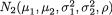
with –∞ < µ1, µ2 < ∞, 0 <  < ∞ and –1 < ρ < 1, n ≥ 2. Then,
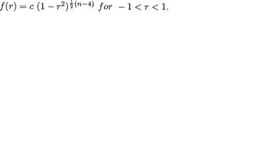
238 4. Functions of Random Variables and Sampling Distribution
by appealing to the Definition 4.6.1 of a multivariate normal distribution, show that
is distributed as  with some ρ*.
{Hint: Look at (4.6.6).}
4.6.9 Suppose that (X1, Y1), ..., (Xn, Yn) are iid 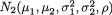 with
with  and –1 < ρ < 1, n ≥ 3. Consider the Pearson correlation coefficient r defined by (4.6.7). The pdf of r when ρ = 0
is given by
where  Use transformation techniques to derive the following result:
4.6.10 Suppose that X1, ..., Xn are iid N2(µ, Σ) where µ 2 and Σ is a 2
×2 p.d. matrix, n ≥ 2. Let us denote  and
and
 Prove the following sampling distributions:
(i) is distributed as N2(µ, n–1 Σ);
(ii)n( – µ)′ Σ–1 (
 – µ) is distributed as
  .
.
{Hint: Apply the Definition 4.6.1 in part (i). To prove part (ii), without any loss of generality, assume that n = 1 and = 0. Now, show that n( – µ)′ Σ–
1 ( – µ) can be written as
 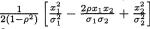 which is further split
up 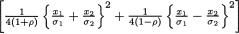 as . At this stage, can the re-
productive property of Chi-squares be applied?}
4.6.11 Suppose that the random vector X, where X′ = (X1, ..., Xp), has a p- dimensional normal distribution with the mean vector 0 and the p × p p.d. dispersion matrix Σ, denoted by Np(0, Σ). We assume that each diagonal entry in Σ is 1. In other words, the (i, j)th entry in the matrix Σ corresponds to the population correlation coefficient ρij between the variables Xi, Xj, 1≤ i ≠ j = p. Suppose that Y is a positive real valued random variable distributed as χν2. It is also assumed that Y and (X1, ..., Xp) are independent. Let us denote p new random variables Ti = Xi ÷ (Y/ν)1/2, i = 1, ..., p. Jointly, however, (T1, ..., Tp) is said to have the p-dimensional t distribution which depends on the correlation matrix Σ, denoted by Mtp(ν, Σ). Assume that Σ–1 exists. Then, show that the joint

4. Functions of Random Variables and Sampling Distribution |
239 |
pdf of T1, ..., Tp, distributed as Mtp(ν, Σ), is given by
with t’ = (t1, ..., tp). {Hint: Start with the joint pdf of X1, ..., Xp and Y. From this, find the joint pdf of T1, ..., Tp and Y by transforming the variables (x1, ..., xp, y) to (t1, ..., tp, y). Then, integrate this latter joint pdf with respect to y.}
4.6.12(Exercise 4.6.5 Continued) Let X1, ..., Xn be iid N(µ, σ2). Recall that Yi = Xi – X1, i = 2, ..., n. Suppose that U is distributed as  and also U is independent of the X’s. Find the joint pdf of Yi/U for i = 2, ..., n.
4.6.13Consider the independent random variables X0, X1, ..., Xp where Xi is distributed as  . We denote the new random variables Ui = νi) ÷ (X0/ν0), i = 1, ..., p. Jointly, (U1, ..., Up) is said to have the p- dimensional F distribution, denoted by MFp(ν0, ν1, ..., νp). Using transformation techniques, show that the joint pdf of U1, ..., Up, distributed as MFp (ν0,
ν1, ..., νp), is given by
with u’ = (u1, ..., up) and  . {Hint: Start with the joint pdf of X0, X1, ..., Xp. From this, find the joint pdf of U1, ..., Up and X0 by transforming (x1, ..., xp, x0) to (u1, ..., up, x0). Then, integrate this latter pdf with respect to x0.}
4.6.14 Suppose that (U1, U2) is distributed as N2(5, 15, 8, 8, ρ) for some
ρ (–1, 1). Let X1 = U1 + U2 and X2 = U1 – U2. Show that X1 and X2 are independently distributed. {Hint: Is (X1, X2) jointly distributed as a bivariate
normal random vector?}
4.7.1 (Examples 3.6.3 and 4.7.1 Continued) Suppose that a pair of random variables (X1, X2) has the joint pdf given by
with 0 < α < 1, where  stands for the bivariate normal pdf defined in (3.6.1) with means µ1, µ2, variances
  , and the correlation coefficient ρ with 0 < ρ < 1. Show that X1 + X2 is not normally
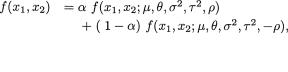
240 4. Functions of Random Variables and Sampling Distribution
distributed. {Hint: Let u = x1 + x2, v = x1 – x2, and find the joint pdf of the transformed random variable (U, V). Integrate this joint pdf with respect to v and show that the marginal pdf of U does not match with the pdf of a normal random variable.}
4.7.2 (Example 3.6.3 and Exercise 4.7.1 Continued) Suppose that a pair of random variables (X1, X2) has the joint pdf given by
with 0 < α < 1, where f(x , x |
; ν, θ, σ2, T2, ρ) stands for the bivariate normal |
|
1 |
2 |
and 0 < ρ < 1. |
pdf defined in (3.6.1) with |
|
|
Show that marginally X1 is N(µ, σ2), X2 is N(θ,T2), but X1 + X2 is not normally distributed.
4.7.3(Example 4.7.2 Continued) Provide the missing details in the Example 4.7.2.
4.7.4If X1, ..., Xn were iid N(µ, σ2) and 
 was the sample variance, then we could claim that (n – 1)S2/σ2 was distributed as a Chi-square random variable with (n–1) degrees of freedom for n ≥
2.Does such a conclusion necessarily need the assumption of the normality or the iid nature of the X sequence? In general there can be different kinds of scenarios on hand. The following problems indicate some of the possibilities. Think through each case carefully and summarize the story each situation unfolds.
(i)Consider Y0, Y1, ..., Yn which are iid N(0, 1), and define then Xi = Yi + Y0, i = 1, ..., n. Obviously,  =
=  + Y0 where
  and
and 
are respectively the sample means of X1, ..., Xn and Y1, ..., Yn. Now,  , which would be distributed as a Chi-square random variable with
(n – 1) degrees of freedom. Note that X1, ..., Xn happen to be normal variables, but these are dependent;
(ii)In part (i), observe that Y0 can be allowed to have any arbitrary distribution while on the other hand Y0 and (Y1, ..., Yn) need not be independent either. Yet, the conclusion that (n – 1)S2 is dis tributed as a Chi-square random variable with (n – 1) degrees of freedom holds. Y0 can even be a discrete random variable!