

 ,
, , as the guess or using
  should be used because
  is sufficient for
 preserves all the information contained in the whole data
 282 6. Sufficiency, Completeness, and Ancillarity
second approach consists of the classical Neyman factorization of a likelihood function. We include specific examples to highlight some approaches to verify whether a statistic is or is not sufficient.
In Section 6.3, the notion of minimal sufficiency is introduced and a fundamental result due to Lehman and Scheffé (1950) is discussed. This result helps us in locating, in some sense, the best sufficient statistic, if it exists. We had seen in Section 3.8 that many standard statistical models such as the binomial, Poisson, normal, gamma and several others belong to an exponential family. It is often a simple matter to locate the minimal sufficient statistic and its distribution in an exponential family. One gets a glimpse of this in the Theorems 6.3.3-6.3.4.
The Section 6.4 provides the idea of quantifying information in both oneand two-parameter situations, but we do so in a fairly elementary fashion. By means of examples, we show that the information contained in the whole data is indeed preserved by the sufficient statistics. In the one-parameter case, we compare the information content in a non-sufficient statistic with that in the data and find the extent of the lost information if a non-sufficient statistic is used as a summary.
The topic of ancillarity is discussed in Section 6.5, again moving deeper into the concepts and highlighting the fact that ancillary statistics can be useful in making statistical inferences. We include the location, scale, and loca- tion-scale families of distributions in Section 6.5.1. The Section 6.6 introduces the concept of completeness and discusses some of the roles complete sufficient statistics play within the realm of statistical inference. Section 6.6.2 highlights Basu’s Theorem from Basu (1955a).
6.2 Sufficiency
Suppose that we start a statistical investigation with observable iid random variables X1, ..., Xn, having a common pmf or pdf f(x), x χ, the domain space for x. Here, n is the sample size which is assumed known. Practically speaking, we like to think that we are going to observe X1, ..., Xn from a population whose distribution is approximated well by f(x). In the example discussed in the introduction, the market analyst is interested in the income distribution of households per month which is denoted by f(x), with some appropriate space χ for x. The income distribution may be indexed by some parameter (or parameter vector) θ (or θ) which captures important features of the distribution. A practical significance of indexing with the parameter θ (or θ) is that once we know the value of θ (or θ), the population distribution f(x) would then be completely specified.

6. Sufficiency, Completeness, and Ancillarity |
283 |
For simplicity, however, let us assume first that θ is a single parameter and denote the population pmf or pdf by f(x; θ) so that the dependence of the features of the underlying distribution on the parameter θ becomes explicit. In classical statistics, we assume that this parameter θ is fixed but otherwise unknown while all possible values of θ Θ, called the parameter space, Θ, the real line. For example, in a problem, we may postulate that the X’s are distributed as N( , σ2) where is the unknown parameter, –∞ < < ∞, but σ(> 0) is known. In this case we may denote the pdf by f(x; θ) with θ = while the parameter space Θ = . But if both the parameters and σ2 are unknown, the population density would be denoted by f(x; θ) where the parameter vector is θ = ( , σ2) Θ = × +. This is the idea behind indexing a population distribution by the unknown parameters in general.
From the context, it should become clear whether the unknown parameter is real valued (θ) or vector valued (θ).
Consider again the observable real valued iid random variables X1, ..., Xn from a population with the common pmf or pdf f(x; θ) where θ( Θ) is the unknown parameter. Our quest for gaining information about the unknown parameter θ can safely be characterized as the core of statistical inference. The data, of course, has all the information about θ even though we have not yet specified how to quantify this “information.” In Section 6.4, we address this. A data can be large or small, and it may be nice or cumbersome, but it is ultimately incumbent upon the experimenter to summarize this data so that all interesting features are captured by its summary. That is, the summary should preferably have the exact same “information” about the unknown parameter θ as does the original data. If one can prepare such a summary, then this would be as good as the whole data as far as the information content regarding the unknown parameter θ is concerned. We would call such a summary sufficient for θ and make this basic idea more formal as we move along.
Definition 6.2.1 Any observable real or vector valued function T ≡ T(X1, ..., Xn), of the random variables X1, ..., Xn is called a statistic.
Some examples of statistics are  , X1 (X2 – Xn:n),
  S2 and so on. As long as the numerical evaluation of T, having observed a specific data
X1 = x1, ..., Xn = xn, does not depend on any unknown quantities, we will call T a statistic. Supposing that X1, ..., Xn are iid N( , σ2) where is unknown, but σ is known, T =  is a statistic because the value of T associated with any observed data x1, ..., xn can be explicitly calculated. In the same example, however, the standardized form of
  , namely

284 6. Sufficiency, Completeness, and Ancillarity
µ)/σ, is not a statistic because it involves the unknown parameter µ, and hence its value associated with any observed data x1, ..., xn can not be calculated.
Definition 6.2.2 A real valued statistic T is called sufficient (for the unknown parameter θ) if and only if the conditional distribution of the random sample X = (X1, ..., Xn) given T = t does not involve θ, for all t  , the domain space for T.
In other words, given the value t of a sufficient statistic T, conditionally there is no more “information” left in the original data regarding the unknown parameter θ. Put another way, we may think of X trying to tell us a story about θ, but once a sufficient summary T becomes available, the original story then becomes redundant. Observe that the whole data X is always sufficient for θ in this sense. But, we are aiming at a “shorter” summary statistic which has the same amount of information available in X. Thus, once we find a sufficient statistic T, we will focus only on the summary statistic T. Before we give other details, we define the concept of joint sufficiency of a vector valued statistic T for an unknown parameter θ.
Definition 6.2.3 A vector valued statistic T ≡ (T1, ..., Tk) where Ti ≡ Ti(X1,
..., Xn), i = 1, ..., k, is called jointly sufficient (for the unknown parameter θ) if and only if the conditional distribution of X = (X1, ..., Xn) given T = t does not involve θ, for all t  k.
k.
The Section 6.2.1 shows how the conditional distribution of X given T = t can be evaluated. The Section 6.2.2 provides the celebrated Neyman factorization which plays a fundamental role in locating sufficient statistics.
6.2.1The Conditional Distribution Approach
With the help of examples, we show how the Definition 6.2.2 can be applied to find sufficient statistics for an unknown parameter θ.
Example 6.2.1 Suppose that X1, ..., Xn are iid Bernoulli(p), where p is the unknown parameter, 0 < p < 1. Here, χ = {0, 1}, θ = p, and Θ = (0, 1). Let us consider the specific statistic  . Its values are denoted by t
  = {0, 1, 2, ..., n}. We verify that T is sufficient for p by showing that the conditional distribution of (X1, ..., Xn) given T = t does not involve p, whatever be t
  . From the Examples 4.2.2-4.2.3, recall that T has the Binomial(n, p) distribution. Now, we obviously have:
But, when  , since
 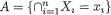 is a subset of B = {T = t},
6. Sufficiency, Completeness, and Ancillarity |
285 |
we can write
Thus, one has
which is free from p. In other words,  is a sufficient statistic for the unknown parameter p. !
Example 6.2.2 Suppose that X1, ..., Xn are iid Poisson(λ) where λ is the unknown parameter, 0 < λ < ∞. Here, χ = {0, 1, 2, ...}, θ = λ, and Θ = (0, ∞). Let us consider the specific statistic  . Its values are denoted by t
 = {0, 1, 2, ...}. We verify that T is sufficient for λ by showing that the conditional distribution of (X1, ..., Xn) given T = t does not involve λ, whatever be t
  . From the Exercise 4.2.2 recall that T has the Poisson(nλ) distribution. Now, we obviously have:
But, when  , since
  is a subset of B = {T = t}, we can write
Hence, one gets
286 6. Sufficiency, Completeness, and Ancillarity
which is free from λ. In other words,  is a sufficient statistic for the unknown parameter λ. !
Example 6.2.3 Suppose that X has the Laplace or double exponential pdf given by f(x; θ) = 1/2θe–|x|/θI(–∞ < x < ∞) where θ (> 0) is an unknown parameter. Let us consider the statistic T = | X |. The difference between X and T is that T provides the magnitude of X, but not its sign. Conditionally given T = t (> 0), X can take one of the two possible values, namely t or –t, each with probability 1/2. In other words, the conditional distribution of X given T = t does not depend on the unknown parameter θ. Hence, | X | is a sufficient statistic for θ. !
Example 6.2.4 Suppose that X1, X2 are iid N(θ, 1) where θ is unknown, – ∞ < θ < ∞. Here, χ = and Θ = . Let us consider the specific statistic T = X1 + X2. Its values are denoted by t  = . Observe that the conditional pdf
of (X1, X2), at (x1, x2) would be zero if x1 + x2 ≠ t when T = t has been observed. So we may work with data points (x1, x2) such that x1 + x2 = t once
T = t is observed. Given T = t, only one of the two X’s is a free-standing variable and so we will have a valid pdf of one of the X’s. Let us verify that T is sufficient for θ by showing that the conditional distribution of X1 given T = t does not involve θ. Now following the Definition 4.6.1 of multivariate normality and the Example 4.6.1, we can claim that the joint distribution of (X1, T) is N2(θ, 2θ, 1, 2,  ), and hence the conditional distribution of X1 given
T = t is normal with its mean = θ +  = 1/2t and conditional
variance = 1 – (  )2 = 1/2, for all t . Refer to the Theorem 3.6.1 for the expressions of the conditional mean and variance. This conditional distribution is clearly free from θ. In other words, T is a sufficient statistic for θ. !
How can we show that a statistic is not sufficient for θ?
Discussions follow.
If T is not sufficient for θ, then it follows from the Definition 6.2.2 that the conditional pmf or pdf of X1, ..., Xn given T = t must depend on the unknown parameter θ, for some possible x1, ..., xn and t.
In a discrete case, suppose that for some chosen data x1, ..., xn, the conditional probability P{X1 = x1, ..., Xn = xn | T = t}, involves the parameter θ. Then, T can not be sufficient for θ. Look at Examples 6.2.5 and 6.2.7.
Example 6.2.5 (Example 6.2.1 Continued) Suppose that X1, X2, X3 are iid Bernoulli(p) where p is unknown, 0 < p < 1. Here, χ = {0, 1}, θ = p,
6. Sufficiency, Completeness, and Ancillarity |
287 |
and Θ = (0, 1). We had verified that the statistic  was sufficient
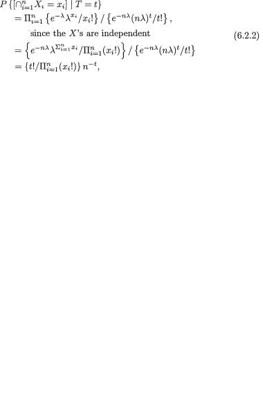
for θ. Let us consider another statistic U = X1X2 + X3. The question is whether U is a sufficient statistic for p. Observe that
Now, since {X1 = 1 n X2 = 0 n X3 = 0} is a subset of {U = 0}, we have
This conditional probability depends on the true value of p and so we claim that the statistic U is not sufficient for p. That is, after the completion of the n trials of the Bernoulli experiment, if one is merely told the observed value of the statistic U, then some information about the unknown parameter p would be lost.!
In the continuous case, we work with the same basic idea. If for some data x1, ..., xn, the conditional pdf given T = t,
fX|T=t(x1, ..., xn), involves the parameter θ, then the statistic T can not be sufficient for θ. Look at the Example 6.2.6.
Example 6.2.6 (Example 6.2.4 Continued) Suppose that X1, X2 are iid N(θ, 1) where θ is unknown, –∞ < θ < ∞. Here, χ = and Θ = . Let us consider a statistic, for example, T = X1 + 2X2 while its values are denoted by t  = . Let us verify that T is not sufficient for θ by showing that the conditional distribution of X1 given T = t involves θ. Now, following the Definition 4.6.1 and the Example 4.6.1, we can claim that the joint distribution of (X1, T) is N2(θ, 3θ, 1, 5,
  ), and hence the conditional distribu-
tion of X1 given T = t is normal with its mean = θ + 
 (t – 3θ) = 1/5(t + 2θ) and variance = 1 – (
  )2 = 4/5, for t . Refer to the Theorem 3.6.1 as needed. Since this conditional distribution depends on the unknown parameter θ, we conclude that T is not sufficient for θ. That
288 6. Sufficiency, Completeness, and Ancillarity
is, merely knowing the value of T after the experiment, some information about the unknown parameter θ would be lost. !
Example 6.2.7 Suppose that X has the exponential pdf given by f(x) = λe– λxI(x > 0) where λ(> 0) is the unknown parameter. Instead of the original data, suppose that we are only told whether X ≤ 2 or X > 2, that is we merely observe the value of the statistic T ≡ I(X > 2). Is the statistic T sufficient for λ? In order to check, let us proceed as follows: Note that we can express P{X > 3 | T = 1} as
which depends on λ and hence T is not a sufficient statistic for λ. !
The methods we pursued in the Examples 6.2.1-6.2.7 closely followed the definition of a sufficient statistic. But, such direct approaches to verify the sufficiency or non-sufficiency of a statistic may become quite cumbersome. More importantly, in the cited examples we had started with specific statistics which we could eventually prove to be either sufficient or nonsufficient by evaluating appropriate conditional probabilities. But, what is one supposed to do in situations where a suitable candidate for a sufficient statistic can not be guessed readily? A more versatile technique follows.
6.2.2The Neyman Factorization Theorem
Suppose that we have at our disposal, observable real valued iid random variables X1, ..., Xn from a population with the common pmf or pdf f(x; θ). Here, the unknown parameter is θ which belongs to the parameter space Θ.
Definition 6.2.4 Consider the (observable) real valued iid random variables X1, ..., Xn from a population with the common pmf or pdf f(x; θ), where the unknown parameter θ Θ. Once we have observed Xi = xi, i = 1, ..., n, the likelihood function is given by
In the discrete case, L(θ) stands for Pθ{X1 = x1 ∩ ... ∩ Xn = xn}, that is the probability of the data on hand when θ obtains. In the continuous case, L(θ) stands for the joint pdf at the observed data point (x1, ..., xn) when θ obtains.
It is not essential however for the X’s to be real valued or that they be iid. But, in many examples, they will be so. If the X’s happen to be vector valued or if they are not iid, then the corresponding joint pmf or pdf of
6. Sufficiency, Completeness, and Ancillarity |
289 |
Xi = xi, i = 1, ..., n, would stand for the corresponding likelihood function L(θ). We will give several examples of L(θ) shortly.
One should note that once the data {xi; i = 1, ..., n} has been observed, there are no random quantities in (6.2.4), and so the likelihood L(.) is simply treated as a function of the unknown parameter θ alone.
The sample size n is assumed known and fixed before the data collection begins.
One should note that θ can be real or vector valued in this general discussion, however, let us pretend for the time being that θ is a real valued parameter. Fisher (1922) discovered the fundamental idea of factorization. Neyman (1935a) rediscovered a refined approach to factorize the likelihood function in order to find sufficient statistics for θ. Halmos and Savage (1949) and Bahadur (1954) gave more involved measure-theoretic treatments.
Theorem 6.2.1 (Neyman Factorization Theorem) Consider the likelihood function L(θ) from (6.2.4). A real valued statistic T = T(X1, ..., Xn) is sufficient for the unknown parameter θ if and only if the following factorization holds:
where the two functions g(.; θ) and h(.) are both nonnegative, h(x1, ..., xn) is free from θ, and g(T(x1, ..., xn);θ) depends on x1, ..., xn only through the observed value T(x1, ..., xn) of the statistic T.
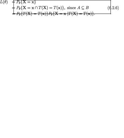
Proof For simplicity, we will provide a proof only in the discrete case. Let
us write X = (X1, ..., Xn) and x = (x1, ..., xn). Let the two sets A and B respectively denote the events X = x and T(X) = T(x), and observe that A B.
Only if part: Suppose that T is sufficient for θ. Now, we write
Comparing (6.2.5)-(6.2.6), let us denote g(T(x1, ..., xn);θ) = Pθ{T(X) = T(x)}
and h(x1, ..., xn) = Pθ{X = x |T(X) = T(x)}. But, we have assumed that T is sufficient for θ and hence by the Definition 6.2.2 of sufficiency, the condi-
tional probability Pθ{X = x |T(X) = T(x)} cannot depend on the parameter θ. Thus, the function h(x1, ..., xn) so defined may depend only on x1, ..., xn. The factorization given in (6.2.5) thus holds. The “only if” part is now complete.¿
290 6. Sufficiency, Completeness, and Ancillarity
If part: Suppose that the factorization in (6.2.5) holds. Let us denote the pmf of T by p(t; θ). Observe that the pmf of T is given by p(t; θ) = Pθ{T(X)
= t} =  . It is easy to see that
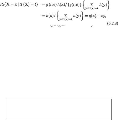
For all x χ such that T(x) = t and p(t; θ) ≠ 0, we can express Pθ{X = x |T(X) = t} as
because of factorization in (6.2.5). Hence, one gets
where q(x) does not depend upon θ. Combining (6.2.7)-(6.2.8), the proof of the “if part” is now complete. !
In the statement of the Theorem 6.2.1, notice that we do not demand that g(T(x1, ..., xn);θ) must be the pmf or the pdf of T(X1, ..., Xn). It is essential, however, that the function h(x1, ..., xn) must be entirely free from θ.
It should be noted that the splitting of L(θ) may not be unique, that is there may be more than one way to determine the function h(.) so that (6.2.5) holds. Also, there can be different versions of the sufficient statistics.
Remark 6.2.1 We mentioned earlier that in the Theorem 6.2.1, it was not essential that the random variables X1, ..., Xn and the unknown parameter θ be all real valued. Suppose that X1, ..., Xn are iid p-dimensional random variables with the common pmf or pdf f(x; θ) where the unknown parameter θ is vector valued, θ Θ q. The Neyman Factorization Theorem can be stated under this generality. Let us consider the likelihood function, 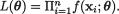
6. Sufficiency, Completeness, and Ancillarity |
291 |
Example 6.2.8 (Example 6.2.1 Continued) Suppose that X1, ..., Xn are iid Bernoulli(p) where p is unknown, 0 < p < 1. Here, χ = {0, 1}, θ = p, and Θ = (0, 1). Then,
which looks like the factorization provided in (6.2.5) where 
 and h(x1, ..., xn) = 1 for all x1, ..., xn {0, 1}. Hence, the statistic T = T(X1, ..., Xn) =
  is sufficient for p. From (6.2.10), we
could instead view L(θ) = g(x1, ..., xn; p) h(x1, ..., xn) with, say, g(x1, ..., xn; p) =  and h(x1, ..., xn) = 1. That is, one could claim that X =
(X1, ..., Xn) was sufficient too for p. But,  provides a significantly reduced summary compared with X, the whole data. We will have more to say on this in the Section 6.3.!
Example 6.2.9 (Example 6.2.2 Continued) Suppose that X1, ..., Xn are iid Poisson(λ) where λ is unknown, 0 < λ < ∞. Here, χ = {0, 1, 2, ...}, θ = λ, and Θ = (0, ∞). Then,
which looks like the factorization provided in (6.2.5) with 
 and h(x1, ..., xn) =
  for all x1, ..., xn {0, 1, 2, ...}. Hence, the statistic T = T(X1, ..., Xn) =
  is sufficient for λ. Again, from
(6.2.11) one can say that the whole data X is sufficient too, but  provides a significantly reduced summary compared with X. !
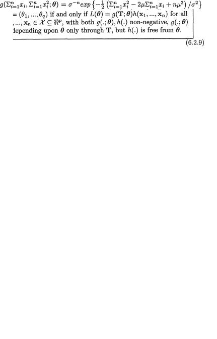
Example 6.2.10 Suppose that X1, ..., Xn are iid N( , σ2) where and σ are both assumed unknown, –∞ < < ∞, 0 < σ < ∞. Here, we may denote θ = ( , σ) so that χ = and Θ = × +. We wish to find jointly sufficient statistics for θ. Now, we have
which looks like the factorization provided in (6.2.9) where one writes and

292 6. Sufficiency, Completeness, and Ancillarity
h(x1, ..., xn) =  for all (x1, ..., xn) n. In other words, T = T(X1, ..., Xn) =
  is jointly sufficient for ( , σ2). !
If T is a sufficient statistic for θ, then any statistic T’ which is a one-to-one function of T is also sufficient for θ.
Example 6.2.11 (Example 6.2.10 Continued) We have  ,
,  , and so it is clear that the transformation from
  to T’ = (
 , S2) is one-to-one. Hence, in the Example 6.2.10, we can also claim that (
 , S2) is jointly sufficient for θ = ( , σ2). !
Let us emphasize another point. Let T be a sufficient statistic for θ. Consider another statistic T’, an arbitrary function of T. Then, the statistic T’ itself is not necessarily sufficient for θ.
Look at the earlier Example 6.2.7.
An arbitrary function of a sufficient statistic T need not be sufficient for θ. Suppose that X is distributed as N(θ, 1) where –∞ < θ < ∞ is the unknown parameter. Obviously, T = X is sufficient for θ. One should check that the statistic T’ = | X |, a function of T, is not sufficient for θ.
Remark 6.2.2 In a two-parameter situation, suppose that the Neyman factorization (6.2.9) leads to a statistic T = (T1, T2) which is jointly sufficient for θ = (θ1, θ2). But, the joint sufficiency of T should not be misunderstood to imply that T1 is sufficient for θ1 or T2 is sufficient for θ2.
From the joint sufficiency of the statistic T = (T1, ..., Tp) for θ = (θ1, ..., θp), one should not be tempted to claim that the
statistic Ti is componentwise sufficient for θi, i = 1, ..., p. Look at the Example 6.2.12. In some cases, the statistic T and θ may not even have the same number of components!
Example 6.2.12 (Example 6.2.11 Continued) In the N( , σ2) case when both the parameters are unknown, recall from the Example 6.2.11 that ( , S2) is jointly sufficient for ( , σ2). This is very different from trying to answer a question like this: Is
  sufficient for or is S2 sufficient for σ2? We can legitimately talk only about the joint sufficiency of the statistic (
 , S2) for θ = ( , σ2).
6. Sufficiency, Completeness, and Ancillarity |
293 |
To appreciate this fine line, let us think through the example again and pretend for a moment that one could claim componentwise sufficiency. But, since ( , S2) is jointly sufficient for ( , σ2), we can certainly claim that (S2,
  ) is also jointly sufficient for θ = ( , σ2). Now, how many readers would be willing to push forward the idea that componentwise, S2 is sufficient for or
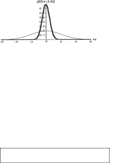
  is sufficient for σ2! Let us denote U =
  and let g(u; n) be the pdf of U when the sample size is n.
Figure 6.2.1. Two PDF’s of Where n = 16
In the Figure 6.2.1, the two pdf’s of  when = 0 and n = 16, for example, are certainly very different from one another. Relatively speaking, the darker pdf gives the impression that σ is “small” whereas the lighter pdf gives the impression that σ is “large”. There should be no doubt that
  provides some information about σ2. In fact
  has some information about both and σ2, whereas S2 has information about σ2 alone. !
Example 6.2.13 Suppose that X1, ..., Xn are iid Uniform(0, θ), where θ (> 0) is unknown. Here, χ = (0, θ) and Θ = +. We wish to find a sufficient statistic for θ. Now,
where xn:1 and xn:n are respectively the observed smallest and largest order statistics. The last step in (6.2.13) looks exactly like the Neyman factorization
provided in (6.2.5) where g(xn:n; θ) = θ–n I (0 < xn:n < θ) and h(x1, ..., xn) = I(0 < xn:1 < xn:n) for all x1, ..., xn (0, θ). Hence, the statistic T = T(X1, ..., Xn) = Xn:n is sufficient for θ. !
It is not crucial that the X’s be iid for the Neyman factorization of the likelihood function to lead to a (jointly) sufficient statistic (T)T. Look at the Example 6.2.14.
294 6. Sufficiency, Completeness, and Ancillarity
In many examples and exercises the X’s are often assumed iid. But, if the X’s are not iid, then all we have to do is to carefully write down the likelihood function L(θ) as the corresponding joint pmf or pdf of the random variables X1, ..., Xn. The Neyman factorization would then hold.
Example 6.2.14 Suppose that X1, X2 are |
independent random variables, |
||||||
with their respective pdf’s f(x |
; θ) = θe–θx |
1 |
I(0 |
< x |
1 |
< ∞) and g(x |
; θ) = 2θe–2θx |
1 |
|
|
|
2 |
2 |
||
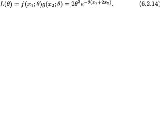
I(0 < x2 < ∞), where θ > 0 is an unknown parameter. For 0 < x1, x2 < ∞, the likelihood function is given by the joint pdf, namely
From (6.2.14) it is clear that the Neyman factorization holds and hence the statistic T = X1 + 2X2 is sufficient for θ. Here, X1, X2 are not identically distributed, and yet the factorization theorem has been fruitful.!
The following result shows a simple way to find sufficient statistics when the pmf or the pdf belongs to the exponential family. Refer back to the Section 3.8 in this context. The proof follows easily from the factorization (6.2.9) and so we leave it out as the Exercise 6.2.15.
Theorem 6.2.2 (Sufficiency in the Exponential Family) Suppose that X1, ..., Xn are iid with the common pmf or the pdf belonging to the k-param- eter exponential family defined by (3.8.4), namely
with appropriate forms for g(x) ≥ 0, a(θ) ≥ 0, bi(θ) and Ri(x), i = 1, ..., k. Suppose that the regulatory conditions stated in (3.8.5) hold. Denote the statistic  j = 1, ..., k. Then, the statistic T = (T1, ..., Tk) is jointly sufficient for θ.
The sufficient statistics derived earlier in the Examples 6.2.8-6.2.11 can also be found directly by using the Theorem 6.2.2. We leave these as the Exercise 6.2.14.
6.3 Minimal Sufficiency
We noted earlier that the whole data X must always be sufficient for the unknown parameter θ. But, we aim at reducing the data by means of summary statistics in lieu of considering X itself. From the series of examples 6.2.8-6.2.14, we found that the Neyman factorization provided sufficient
 , the median (
 ,
,  or
or  1/2 ( +
  ,
,  ,
, 296 6. Sufficiency, Completeness, and Ancillarity
between a statistic and so called partitions it induces on the sample space.
Let us look at the original data X = (X1, ..., Xn) where x = (x1, ..., xn) χn. Consider a statistic T ≡ T(X1, ..., Xn), that is T is a mapping from χn onto some
space  say. For t
  , let χt = {x : x χn such that T(x) = t} which are disjoint subsets of χn and also χn = ?t χt. In other words, the collection of
subsets {χt : t  } forms a partition of the space χn. Often, {χt : t
  } is also called the partition of χn induced by the statistic T.
Theorem 6.3.1 (Minimal Sufficient Statistics) Let us consider the function  , the ratio of the likelihood functions from (6.2.9) at x and y, where θ is the unknown parameter and x, y χn. Suppose that we have a statistic T ≡ T(X1, ..., Xn) = (T1, ..., Tk) such that the following conditions hold:
Then, the statistic T is minimal sufficient for the parameter θ.
Proof We first show that T is a sufficient statistic for θ and then we verify that T is also minimal. For simplicity, let us assume that f(x; θ) is positive for all x χn and θ.
Sufficiency part: Start with {χt : t  } which is the partition of χn induced by the statistic T. In the subset χt, let us select and fix an element xt. If we look at an arbitrary element x χn, then this element x belongs to χt for some unique t so that both x and xt belong to the same set χt. In other words, one has T(x) = T(xt). Thus, by invoking the “if part” of the statement in (6.3.1), we can claim that h(x, xt; θ) is free from θ. Let us then denote h(x) ≡ h(x, xt; θ), x χn. Hence, we write
where xt = (xt1, ..., xtn). In view of the Neyman Factorization Theorem, the statistic T(x) is thus sufficient for θ.¿
Minimal part: Suppose U = U(X) is another sufficient statistic for θ. Then, by the Neyman Factorization Theorem, we can write
6. Sufficiency, Completeness, and Ancillarity |
297 |
for some appropriate g0(.; θ) and h0(.). Here, h0(.) does not depend upon θ. Now, for any two sample points x = (x1, ..., xn), y = (y1, ..., yn) from χn such that U(x) = U(y), we obtain
Thus, h(x, y; θ) is free from θ. Now, by invoking the “only if” part of the statement in (6.3.1), we claim that T(x) = T(y). That is, T is a function of U. Now, the proof is complete. !
Example 6.3.1 (Example 6.2.8 Continued) Suppose that X1, ..., Xn are iid Bernoulli(p), where p is unknown, 0 < p < 1. Here, χ = {0, 1}, θ = p, and Θ = (0, 1). Then, for two arbitrary data points x = (x1, ..., xn) and y = (y1, ..., yn), both from χ, we have:
From (6.3.2), it is clear that  would become free
from the unknown parameter p if and only if  , that is, if and only if
  Hence, by the theorem of Lehmann-Scheffé, we claim that
  is minimal sufficient for p. !
We had shown non-sufficiency of a statistic U in the Example 6.2.5. One can arrive at the same conclusion by contrasting U with
a minimal sufficient statistic. Look at the Examples 6.3.2 and 6.3.5.
Example 6.3.2 (Example 6.2.5 Continued) Suppose that X1, X2, X3 are iid Bernoulli(p), where p is unknown, 0 < p < 1. Here, χ = {0, 1}, θ = p, and Θ = (0, 1). We know that the statistic  is minimal sufficient for p. Let U = X1 X2 + X3, as in the Example 6.2.5, and the question is whether U is a sufficient statistic for p. Here, we prove again that the statistic U can not be sufficient for p. Assume that U is sufficient for p, and then
  must be a function of U, by the Definition 6.3.1 of minimal sufficiency. That is, knowing an observed value of U, we must be able to come up with a unique observed value of T. Now, the event {U = 0}
298 6. Sufficiency, Completeness, and Ancillarity
consists of the union of possibilities such as {X1 = 0 ∩ X2 = 0 ∩ X3 = 0}, {X1
= 0 ∩ X2 = 1 ∩ X3 = 0}, and {X1 = 1 ∩ X2 = 0 ∩ X3 = 0}. Hence, if the event {U = 0} is observed, we know then that either T = 0 or T = 1 must be
observed. But, the point is that we cannot be sure about a unique observed value of T. Thus, T can not be a function of U and so there is a contradiction. Thus, U can not be sufficient for p. !
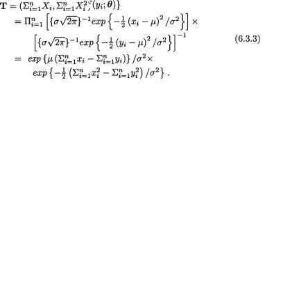
Example 6.3.3 (Example 6.2.10 Continued) Suppose that X1, ..., Xn are iid N( , σ2), where θ = ( , σ) and both , σ are unknown, –∞ < < ∞, 0 < σ < ∞. Here, χ = and Θ = × +. We wish to find a minimal sufficient statistic for θ. Now, for two arbitrary data points x = (x1, ..., xn) and y = (y1, ..., yn), both from χ, we have:
From (6.3.3), it becomes clear that the last expression would not involve the
unknown parameter θ = ( , σ) if and only if |
|
as well as |
|
, |
that is, if and only if |
= |
and |
. Hence, by the theorem of Lehmann-Scheffé, we claim |
|||
that |
is minimal sufficient for ( , σ). ! |
|
|
Theorem 6.3.2 Any statistic which is a one-to-one function of a minimal sufficient statistic is itself minimal sufficient.
Proof Suppose that a statistic S is minimal sufficient for θ. Let us consider another statistic T = h(S) where h(.) is one-to-one. In Section 6.2.2, we mentioned that a one-to-one function of a (jointly) sufficient statistic is (jointly) sufficient and so T is sufficient. Let U be any other sufficient statistic for θ. Since, S is minimal sufficient, we must have S = g(U) for some g(.). Then, we obviously have T = h(S) = h(g(U)) = h  g(U) which verifies the minimality of the statistic T. !
Example 6.3.4 (Example 6.3.3 Continued) Suppose that X1, ..., Xn are iid N( , σ2), where θ = ( , σ) and both , σ are unknown, –∞ < < ∞, 0 < σ < ∞. We know that is minimal sufficient for ( , σ). Now, ( , S2) being a one-to-one function of T, we can claim that (
 , S2) is also minimal sufficient. !
Example 6.3.5 (Example 6.3.3 Continued) Suppose that X1, X2, X3 are iid N( , σ2) where is unknown, but σ is assumed known, –∞ < < ∞,
6. Sufficiency, Completeness, and Ancillarity |
299 |
0 < σ < ∞. Here, we write θ = , χ = and Θ = . It is easy to verify that the statistic  is minimal sufficient for θ. Now consider the statistic U = X1 X2 + X3 and suppose that the question is whether U is sufficient for θ. Assume that U is sufficient for θ. But, then
  must be a function of U, by the Definition 6.3.1 of minimal sufficiency. That is, knowing an observed value of U, we must be able to come up with a unique value of T. One can proceed in the spirit of the earlier Example 6.3.2 and easily arrive at a contradiction. So, U cannot be sufficient for θ. !
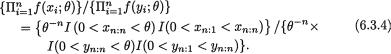
Example 6.3.6 (Example 6.2.13 Continued) Suppose that X1, ..., Xn are iid Uniform(0, θ), where θ (> 0) is unknown. Here, χ = (0, θ) and Θ = +. We wish to find a minimal sufficient statistic for θ. For two arbitrary data points x = (x1, ..., xn) and y = (y1, ..., yn), both from χ, we have:
Let us denote a(θ) = I(0 < xn:n < θ)/I(0 < yn:n < θ). Now, the question is this: Does the term a(θ) become free from θ if and only if xn:n = yn:n?
If we assume that xn:n = yn:n, then certainly a(θ) does not involve θ. It remains to show that when a(θ) does not involve θ, then we must have xn:n =
yn:n. Let us assume that xn:n ≠ yn:n, and then show that a(θ) must depend on the value of θ. Now, suppose that xn:n = 2, yn:n = .5. Then, a(θ) = 0, 1 or 0/0 when θ = 1, 3 or .1 respectively. Clearly, a(θ) will depend upon the value of θ
whenever xn:n ≠ yn:n. We assert that the term a(θ) becomes free from θ if and only if xn:n = yn:n. Hence, by the theorem of Lehmann-Scheffé, we claim that
T = Xn:n, the largest order statistic, is minimal sufficient for θ. !
Remark 6.3.1 Let X1, ..., Xn be iid with the pmf or pdf f(x; θ), x χ ,
θ = (θ1, ..., θk) Θ k. Suppose that a statistic T = T(X) = (T1(X), ..., Tr(X)) is minimal sufficient for θ. In general can we claim that r = k? The
answer is no, we can not necessarily say that r = k. Suppose that f(x; θ) corresponds to the pdf of the N(θ, θ) random variable with the unknown parameter θ > 0 so that k = 1. The reader should verify that  is a minimal sufficient for θ so that r = 2. Here, we have r > k. On the other hand, suppose that X1 is N( , σ2) where and σ2 are both unknown parameters. In this case one has θ = ( , σ2) so that k = 2. But, T = X1 is minimal sufficient so that r = 1. Here, we have r < k. In many situations, of course, one would find that r = k. But, the point is that there is no guarantee that r would necessarily be same as k.
The following theorem provides a useful tool for finding minimal sufficient
300 6. Sufficiency, Completeness, and Ancillarity
statistics within a rich class of statistical models, namely the exponential family. It is a hard result to prove. One may refer to Lehmann (1983, pp. 43-44) or Lehmann and Casella (1998) for some of the details.
Theorem 6.3.3 (Minimal Sufficiency in the Exponential Family) Suppose that X1, ..., Xn are iid with the common pmf or the pdf belonging to the k-parameter exponential family defined by (3.8.4), namely
with some appropriate forms for g(x) ≥ 0, a(θ) ≥ 0, bi(θ) and Ri(x), i = 1, ..., k. Suppose that the regulatory conditions stated in (3.8.5) hold. Denote the statistic  . Then, the statistic T = (T1, ..., Tk) is (jointly) minimal sufficient for θ.
The following result provides the nature of the distribution itself of a minimal sufficient statistic when the common pmf or pdf comes from an exponential family. Its proof is beyond the scope of this book. One may refer to the Theorem 4.3 of Lehmann (1983) and Lemma 8 in Lehmann (1986). One may also review Barankin and Maitra (1963), Brown (1964), Hipp (1974), Barndorff-Nielsen (1978), and Lehmann and Casella (1998) to gain broader perspectives.
Theorem 6.3.4 (Distribution of a Minimal Sufficient Statistic in the Exponential Family) Under the conditions of the Theorem 6.3.3, the pmf or the pdf of the minimal sufficient statistic (T1, ..., Tk) belongs to the k-param- eter exponential family.
In each example, the data X was reduced enormously by the minimal sufficient summary. There are situations where no significant data reduction may be possible.
See the Exercise 6.3.19 for specific examples.
6.4 Information
Earlier we have remarked that we wish to work with a sufficient or minimal sufficient statistic T because such a statistic will reduce the data and preserve all the “information” about θ contained in the original data. Here, θ may be real or vector valued. But, how much information do we have in the original data which we are trying to preserve? Now our major concern is to quantify the information content within some data. In order to keep the deliberations simple, we discuss the one-parameter and two-parameter
 (
( . Thus, we have
 . Thus we have
 . Now, utilizing (6.4.1), one can write down the information contained in the data
  for each
6. Sufficiency, Completeness, and Ancillarity |
303 |
Now, let us write
so that 0 =  dx. Hence one obtains
Next, combining (6.4.6)-(6.4.8), we conclude that IX(θ) = nIX1(θ). !
Suppose that we have collected random samples X1, ..., Xn from a population and we have evaluated the information IX(θ) contained in the data X = (X1, ..., Xn). Next, suppose also that we have a statistic T = T(X) in mind for which we have evaluated the information IT(θ) contained in T. If it turns out that IT(θ), can we then claim that the statistic T is indeed sufficient for θ? The answer is yes, we certainly can. We state the following result without supplying its proof. One may refer to Rao (1973, result (iii), p. 330) for details. In a recent exchange of personal communications, C. R. Rao has provided a simple way to look at the Theorem 6.4.2. In the Exercise 6.4.15, we have given an outline of Rao’s elegant proof of this result. In the Examples 6.4.3-6.4.4, we find opportunities to apply this theorem.
Theorem 6.4.2 Suppose that X is the whole data and T = T(X) is some statistic. Then, IX(θ) ≥ IT(θ) for all θ Θ. The two information measures match with each other for all θ if and only if T is a sufficient statistic for θ.
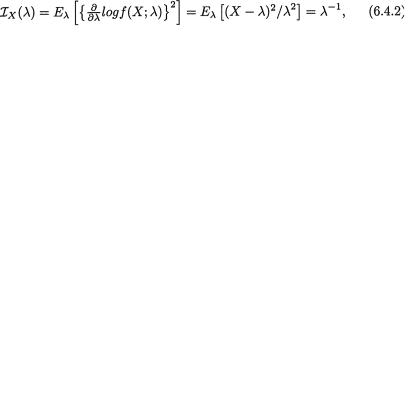
Example 6.4.3 (Example 6.4.1 Continued) Suppose that X1, ..., Xn are iid Poisson(λ), where λ (> 0) is the unknown parameter. We already know that  is a minimal sufficient statistic for λ and T is distributed as Poisson(nλ). But, let us now pursue T from the information point of view. One can start with the pmf g(t; λ) of T and verify that
as follows: Let us write log{g(t; λ)} = –nλ+tlog(nλ) – log(t!) which implies
that  log{g(t;λ)} = –n + tλ-1. So, IT(λ) = Eλ [{
 log{g(T;λ)}}2] = Eλ [(T - nλ)2/λ2] = nλ-1 since Eλ[(T - nλ)2] = V(T) = nλ.
On the other hand, from (6.4.4) and Example 6.4.1, we can write IX(λ) = nIX1(λ) = nλ-1. That is, T preserves the available information from the whole data X. The Theorem 6.4.2 implies that the statistic T is indeed sufficient for λ . !
 was sufficient for . Let us now pursue
 =
=  is finite for all
  is finite for all
 = –
= – 

6. Sufficiency, Completeness, and Ancillarity |
305 |
we only discuss the case of a two-dimensional parameter. Suppose that X is an observable real valued random variable with the pmf or pdf f(x;θ) where the parameter θ = (θ1, θ2) Θ, an open rectangle 2, and the χ space does
not depend upon θ. We assume throughout that |
f(x; θ) exists, i = 1, 2, for |
all x χ, θ Θ, and that we can also interchange the partial derivative (with respect to θ1, θ2) and the integral (with respect to x).
Definition 6.4.2 Let us extend the earlier notation as follows. Denote
Iij(θ) = Eθ  , for i, j = 1, 2. The Fisher information matrix or simply the information matrix about θ is given by
Remark 6.4.2 In situations where |
f(x; θ) exists for all x χ, for all |
i, j = 1, 2, and for all θ Θ, we can alternatively write
and express the information matrix IX(θ) accordingly. We have left this as an exercise.
Having a statistic T = T(X1, ..., Xn), however, the associated information matrix about θ will simply be calculated as IT(θ) where one would replace the original pmf or pdf f(x; θ) by that of T, namely g(t;θ), t  . When we compare two statistics T1 and T2 in terms of their information content about a single unknown parameter θ, we simply look at the two one-dimensional quantities IT1 (θ) and IT2 (θ), and compare these two numbers. The statistic associated with the larger information content would be more appealing. But, when θ is two-dimensional, in order to compare the two statistics T1 and T2, we have to consider their individual two-dimensional information matrices IT1(θ) and IT2(θ). It would be tempting to say that T1 is more informative about θ than T2 provided that
 so that
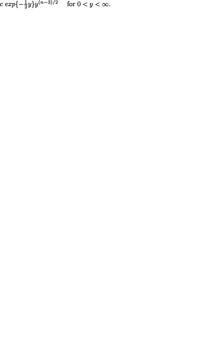
 is distributed as
  . Utilizing (6.4.18), we obtain the following information matrix corresponding to the statistic
  :
: , then there is some loss of information. In other words,
  does not preserve all the information contained in the data
  . We are aware that
  for
for 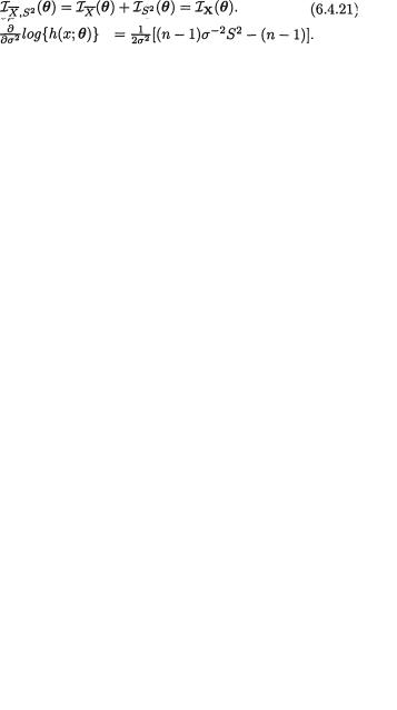
308 6. Sufficiency, Completeness, and Ancillarity
so that one has
Hence we obtain
Obviously, I12(θ) = I21(θ) = 0 corresponding to S2. Utilizing (6.4.21), we obtain the information matrix corresponding to the statistic S2, namely,
Comparing (6.4.17) and (6.4.22), we observe that
which is a positive semi definite matrix. That is, if we summarize the whole data X only through S2, then there is certainly some loss of information whenand σ2 are both assumed unknown. !
Example 6.4.10 (Examples 6.4.8-6.4.9 Continued) Individually, whether we consider the statistic  or S2, both lose some information in comparison with IX(θ), the information contained in the whole data X. This is clear from (6.4.20) and (6.4.23). But recall that
  and S2 are independently distributed, and hence we note that
That is, the lost information when we consider only  or S2 is picked up by the other statistic. !
In the Example 6.4.10, we tacitly used a particular result which is fairly easy to prove. For the record, we merely state this result while its proof is left as the Exercise 6.4.11.
Theorem 6.4.3 Suppose that X1, ..., Xn are iid with the common pmf or pdf given by f(x; θ). We denote the whole data X = (X1, ..., Xn). Suppose that we have two statistics T1 = T1(X), T2 = T2(X) at our disposal and T1, T2 are distributed independently. Then, the information matrix IT(θ) is given by
6. Sufficiency, Completeness, and Ancillarity |
309 |
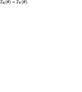
Let us now go back for a moment to (6.4.10) for the definition of the information matrix IX(θ). Now suppose that Y = h(X) where the function h(.) : χ → Y is one-to-one. It should be intuitive enough to guess that IX(θ) = IY(θ). For the record, we now state this result formally.
Theorem 6.4.4 Let X be an observable random variable with its pmf or pdf f(x; θ) and the information matrix IX(θ). Suppose that Y = h(X) where the function h(.) : χ → Y is one-to-one. Then, the information matrix about the unknown parameter θ contained in Y is same as that in X, that is
Proof In order to keep the deliberations simple, we consider only a real valued continuous random variable X and a real valued unknown parameter θ.
Recall that we can write 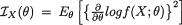 . Note that x = h-1(y)
is well-defined since h(.) is assumed one-to-one. Now, using the transformation techniques from (4.4.1), observe that the pdf of Y can be expressed as
Thus, one immediately writes
The vector valued case and the case of discrete X can be disposed off with minor modifications. These are left out as Exercise 6.4.12. !
6.5 Ancillarity
The concept called ancillarity of a statistic is perhaps the furthest away from sufficiency. A sufficient statistic T preserves all the information about θ contained in the data X. To contrast, an ancillary statistic T by itself provides no information about the unknown parameter θ. We are not implying that an ancillary statistic is necessarily bad or useless. Individually, an ancillary statistic would not provide any information about θ, but
310 6. Sufficiency, Completeness, and Ancillarity
such statistics can play useful roles in statistical methodologies. In the mid 1920’s, R. A. Fisher introduced this concept and he frequently revisited it in his writings. This concept evolved from Fisher (1925a) and later it blossomed into the vast area of conditional inferences. In his 1956 book, Fisher emphasized many positive aspects of ancillarity in analyzing real data. Some of these ideas will be explored in this and the next section. For fuller discussions of conditional inference one may look at Basu (1964), Hinkley (1980a) and Ghosh (1988). The interesting article of Reid (1995) also provides an assessment of conditional inference procedures.
Consider the real valued observable random variables X1, ..., Xn from some population having the common pmf or pdf f(x; θ), where the unknown parameter vector θ belongs to the parameter space Θ p. Let us continue writing X = (X1, ..., Xn) for the data, and denote a vector valued statistic by T = T(X).
Definition 6.5.1 A statistic T is called ancillary for θ or simply ancillary provided that the pmf or the pdf of T, denoted by g(t) for t  , does not involve the unknown parameter θ Θ.
Example 6.5.1 Suppose that X1, ..., Xn are iid N(θ, 1) where θ is the unknown parameter, –∞ < θ < ∞, n ≥ 3. A statistic T1 = X1 – X2 is distributed as N(0, 2) whatever be the value of the unknown parameter θ. Hence T1 is ancillary for θ. Another statistic T2 = X1 + ... + Xn–1 – (n – 1)Xn is distributed as N(0, n(n – 1)) whatever be the value of the unknown parameter θ. Hence
T2 is also ancillary for θ. The sample variance S2 is distributed as  whatever be the value of the unknown parameter θ and hence S2 is ancillary too for θ. !
Example 6.5.2 Suppose that X1, ..., Xn are iid N( , σ2), θ = ( , σ2), –∞ << ∞, 0 < σ2 < ∞, n ≥ 2. Here both the parameters and σ are assumed unknown. Let us reconsider the statistics T1 or T2 defined in the Example 6.5.1. Now, T1, T2 are respectively distributed as N(0, 2σ2) and N(0, n(n – 1)σ2) respectively, and both these distributions clearly depend upon θ. Thus, T1 or T2 is no longer ancillary for θ in this situation. The sample variance S2 is
distributed as |
and hence S2 is not ancillary either for θ. But, |
consider another statistic T3 = (X1 – X2)/S where S2 is the sample variance. Denoting Yi = (Xi – )/σ, observe that in terms of the Y’s, we can equivalently rewrite T32 as
Since Y1, ..., Yn are iid N(0, 1), starting with the likelihood function of Y = (Y1, ..., Yn), and then by using transformations, one can find the pdf of U3. We leave it as an exercise. But, since the likelihood function of Y would not

6. Sufficiency, Completeness, and Ancillarity |
311 |
involve θ to begin with, the pdf of U3 would not involve θ. In other words, T3 is an ancillary statistic here. Note that we do not need the explicit pdf of U3 to conclude this. !
In Example 6.5.2, note that  has a Student’s t distribution with (n - 1) degrees of freedom which is free from θ. But, we do not talk about its ancillarity or non-ancillarity since T4 is not a statistic. T3, however, was a statistic. The expression used in (6.5.1) was merely a device to argue that the distribution
of the statistic T3 in the Example 6.5.2 was free from θ.
Example 6.5.3 Suppose that X1, ..., Xn are iid with the common pdf f(x; λ) = λe–λx I(x > 0) where λ(> 0) is the unknown parameter with n = 2. Let us
write S2 = (n - 1)-1  and denote
  T1 = X1/Xn, T2 = X2/U, T3 = (X1 + X3)/S. Define Yi = λXi for i = 1, ..., n and it is obvious that the
joint distribution of Y = (Y1, ..., Yn) does not involve the unknown parameter λ. Next, one can rewrite the statistic T1 as Y1/Yn and its pdf cannot involve λ.
So, T1 is ancillary. Also, the statistic T2 can be rewritten as Y2/{ Yi} and its pdf cannot involve λ. So, T2 is ancillary. Similarly one can argue that T3 is also ancillary. The details are left out as Exercise 6.5.2. !
Example 6.5.4 (Example 6.5.1 Continued) Suppose that X1, X2, X3 are iid N(θ, 1) where θ is the unknown parameter, –∞ < θ < ∞. Denote T1 = X1 - X2, T2 = X1 + X2 - 2X3, and consider the two dimensional statistic T = (T1, T2). Note that any linear function of T1, T2 is also a linear function of X1, X2, X3, and hence it is distributed as a univariate normal random variable. Then, by the Definition 4.6.1 of the multivariate normality, it follows that the statistic T is distributed as a bivariate normal variable. More specifically, one can check that T is distributed as N2(0, 0, 2, 6, 0) which is free from θ. In other words, T is an ancillary statistic for θ. !
Example 6.5.5 (Example 6.5.2 Continued) Suppose that X1, ..., Xn are iid N(µ, σ2), θ = (µ, σ2), –∞ < µ < ∞, 0 < σ2 < ∞, n ≥ 4. Here, both the parameters µ and σ are assumed unknown. Let S2 be the sample variance and
T1 = (X1 - X3)/S, T2 = (X1 + X3 - 2X2)/S, T3 = (X1 – X3 + 2X2 – 2X4)/S, and denote the statistic T = (T1, T2, T3). Follow the technique used in the Example
6.5.2 to show that T is ancillary for θ. !
We remarked earlier that a statistic which is ancillary for the unknown parameter θ can play useful roles in the process of inference making. The following examples would clarify this point.
6. Sufficiency, Completeness, and Ancillarity |
312 |
Example 6.5.6 (Example 6.5.1 Continued) Suppose that X1, X2 are iid N(θ, 1) where θ is the unknown parameter, –∞ < θ < ∞. The statistic T1 = X1 – X2 is ancillary for θ. Consider another statistic T2 = X1. One would recall from Example 6.4.4 that  (θ) = 1 whereas IX(θ) = 2, and so the statistic T2 can not be sufficient for θ. Here, while T2 is not sufficient for θ, it has some information about θ, but T1 itself has no information about θ. Now, if we are told the observed value of the statistic T = (T1, T2), then we can reconstruct the original data X = (X1, X2) uniquely. That is, the statistic T = (T1, T2) turns out to be jointly sufficient for the unknown parameter θ. !
Example 6.5.7 This example is due to D. Basu. Suppose that (X, Y) is a bivariate normal variable distributed as N2(0, 0, 1, 1, ρ), introduced in Section 3.6, where the unknown parameter is the correlation coefficient ρ (–1, 1). Now consider the two statistics T1 = X and T2 = Y. Since T1 and T2 have individually both standard normal distributions, it follows that T1 is ancillary for ρ and so is T2. But, note that the statistic T = (T1, T2) is minimal sufficient for the unknown parameter ρ. What is remarkable is that the statistic T1 has no information about ρ and the statistic T2 has no information about ρ, but the statistic (T1, T2) jointly has all the information about ρ. !
The situation described in (6.5.2) has been highlighted in the Example 6.5.6 where we note that (T1, T2) is sufficient for θ, but (T1, T2) is not minimal sufficient for θ. Instead, 2T2 - T1 is minimal sufficient in the Example 6.5.6. The situation described in (6.5.3) has been highlighted in the Example 6.5.7 where we note especially that (T1, T2) is minimal sufficient for θ. In other words, there are remarkable differences between the situations described by these two Examples.
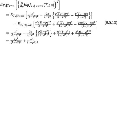
Let us now calculate the information  where ρ is the correlation coefficient in a bivariate normal population.
6. Sufficiency, Completeness, and Ancillarity |
313 |
With  , from (3.6.2), one can write down the joint pdf of (X, Y):
In order to derive the expression for the Fisher information IX,Y(ρ), one may proceed with the natural logarithm of f(x, y; ρ). Next, differentiate the natural logarithm with respect to ρ, followed by squaring it, and then evaluating the expectation of that expression after replacing (x, y) with (X, Y). This direct approach becomes quite involved and it is left as an exercise. Let us, however, adopt a different approach in the following example.
Example 6.5.8 (Example 6.5.7 Continued) Suppose that (X, Y) is distributed as N2(0, 0, 1, 1, ρ), where the unknown parameter is the correlation coefficient ρ (–1, 1). Define U = X - Y, V = X + Y, and notice that (U, V) can be uniquely obtained from (X, Y) and vice versa. In other words,
IU,V(ρ) and IX,Y(ρ) should be exactly same in view of the Theorem 6.4.4. But, observe that (U, V) is distributed as N2(0, 0, 2(1 – ρ), 2(1 + ρ), 0), that is U
and V are independent random variables. Refer back to the Section 3.7 as needed. Hence, using the Theorem 6.4.3, we immediately conclude that IU,V(ρ) = IU(ρ) + IV(ρ). So, we can write:
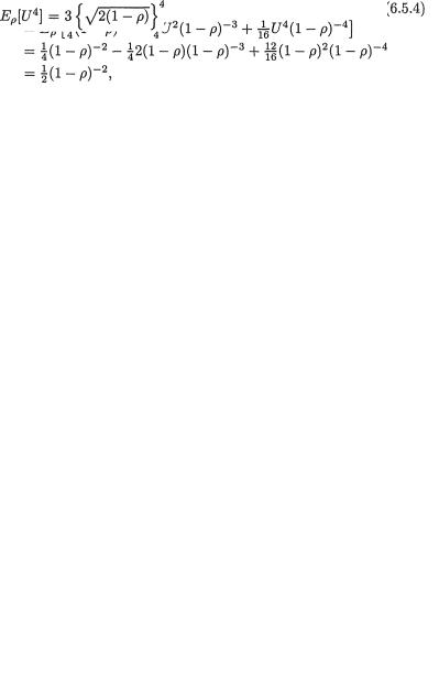
That is, it will suffice to evaluate IU(ρ) and IV(ρ) separately. It is clear that U is N(0, 2(1 – ρ)) while V is N(0, 2(1 + ρ)). The pdf of U is given by
so that one has
Hence, we write
since E [U2] = 2(1 – ρ), |
. Similarly, one would |
ρ |
|
verify that IV(ρ) = ½(1 + ρ)–2. Then, from (6.5.5), we can obviously write:
6. Sufficiency, Completeness, and Ancillarity |
314 |
A direct verification of (6.5.6) using the expression of f(x, y; ρ) is left as the Exercise 6.5.17. !
Example 6.5.9 Let X1, X2, ... be a sequence of iid Bernoulli(p), 0 < p < 1. One may think of Xi = 1 or 0 according as the ith toss of a coin results in a head (H) or tail (T) where P(H) = 1 – P(T) = p in each independent toss, i = 1, ..., n. Once the coin tossing experiment is over, suppose that we are only told how many times the particular coin was tossed and nothing else. That is, we are told what n is, but nothing else about the random samples X1, ..., Xn. In this situation, knowing n alone, can we except to gain any knowledge about the unknown parameter p? Of course, the answer should be “no,” which amounts to saying that the sample size n is indeed ancillary for p. !
6.5.1The Location, Scale, and Location-Scale Families
In Chapter 3, we discussed a very special class of distributions, namely the exponential family. Now, we briefly introduce a few other special ones which are frequently encountered in statistics. Let us start with a pdf g(x), x and construct the following families of distributions defined through the g(.) function:
The understanding is that θ, δ may belong to some appropriate subsets of ,+ respectively. The reader should check that the corresponding members f(.) from the families F1, F2, F3 are indeed pdf’s themselves.
The distributions defined via parts (i), (ii), and (iii) in (6.5.7) are respectively said to belong to the
location, scale, and location-scale family.
We often say that the families F1, F2, F3 are respectively indexed by (i) the parameter θ, (ii) the parameter δ, and (iii) the parameters θ and δ. In part (i) θ is called a location parameter, (ii) δ is called a scale parameter, and (iii) θ, δ are respectively called the location and scale parameters.
For example, the collection of N(µ, 1) distributions, with µ , forms a location family. To see this, let g(x) = φ (x) =  exp{–x2/2}, x
6. Sufficiency, Completeness, and Ancillarity |
315 |
and then write F1 = {f(x; µ) = φ (x – µ) : µ , x }. Next, the collection of N(0, σ2) distributions, with σ +, forms a scale family. To see this, let us simply write F2 = {f(x; σ) = σ–1 φ (x/σ) : σ +, x }. The collection of N(µ, σ2) distributions, with µ , σ +, forms a location-scale family. We
simply write F3 = {f(x; µ, σ) = σ–1 φ ((x – µ)/σ) : µ , σ +, x }. We have left other examples as exercises.
In a location family, the role of the location parameter θ is felt in the “movement” of the pdf along the x-axis as different values of θ are contemplated. The N(0, 1) distribution has its center of symmetry at the point x = 0, but the N(µ, 1) distribution’s center of symmetry moves along the x-axis, to the right or left of x = 0, depending upon whether µ is positive or negative, without changing anything with regard to the shape of the probability density curve. In this sense, the mean µ of the normal distribution serves as a location parameter. For example, in a large factory, we may look at the monthly wage of each employee and postulate that the distribution of wage as N(µ, σ2) where σ = $100. After the negotiation of a new contract, suppose that each employee receives $50 monthly raise. Then the distribution moves to the right with its new center of symmetry at µ + 50. The intrinsic shape of the distribution can not change in a situation like this.
In a scale family, the role of the scale parameter δ is felt in “squeezing or expanding” the pdf along the x-axis as different values of δ are contemplated. The N(0, 1) distribution has its center of symmetry at the point x = 0. The N(0, δ2) distribution’s center of symmetry stays put at the point x = 0, but depending on whether δ is larger or smaller than one, the shape of the density curve will become more flat or more peaked, compared with the standard normal, around the center. In this sense, the variance δ2 of the normal distribution serves as a scale parameter. Suppose that we record the heights (in inches) of individuals and we postulate the distribution of these heights as N(70, σ2). If heights are measured in centimeters instead, then the distribution would appear more spread out around the new center. One needs to keep in mind that recording the heights in centimeters would amount to multiplying each original observation X measured in inches by 2.54.
In a location-scale family, one would notice movement of the distribution along the x-axis as well as the squeezing or expansion effect in the shape. We may be looking at a data on the weekly maximum temperature in a city recorded over a period, in Fahrenheit (F) or Celsius (C). If one postulates a normal distribution for the temperatures, changing the unit of measurements from Fahrenheit to Celsius would amount to shifts in both the origin and scale. One merely needs to recall the relationship 1/5C =
6. Sufficiency, Completeness, and Ancillarity |
316 |
-1 (F - 32) between the two units, Fahrenheit and Celsius.
9
At this point, one may ask the following question. What is the relevance of such special families of distributions in the context of ancillarity? It may help if one goes back to the Examples 6.5.1-6.5.5 and thinks through the process of how we had formed some of the ancillary statistics. Suppose that X1, ..., Xn are iid random variables having the common pdf f(x), indexed by some appropriate parameter(s). Then, we can conclude the following.
One should not, however, get the impression that (6.5.8)-(6.5.10) list the unique or in some sense the “best” ancillary statistics. These summary statements and ancillary statistics should be viewed as building blocks to arrive at many forms of ancillary statistics.
6.5.2Its Role in the Recovery of Information
In Examples 6.5.6-6.5.7, we had seen how ancillary statistics could play significant roles in conjunction with non-sufficient statistics. Suppose that T1 is a non-sufficient statistic for θ and T2 is ancillary for θ. In other words, in terms of the information content,  < IX(θ) where X is the whole data and
  = 0 for all θ Θ. Can we recover all the information contained in X by reporting T1 while conditioning on the observed value of T2? The answer is: we can do so and it is a fairly simple process. Such a process of conditioning has far reaching implications as emphasized by
6. Sufficiency, Completeness, and Ancillarity |
317 |
Fisher (1934, 1956) in the famous “Nile” example. One may also refer to Basu (1964), Hinkley (1980a), Ghosh (1988) and Reid (1995) for fuller discussions of conditional inference.
The approach goes through the following steps. One first finds the conditional pdf of T1 at the point T1 = u given that T2 = v, denoted by  . Using this conditional pdf, one obtains the information content, namely
  following the Definition 6.4.1. In other words,
In general, the expression of  would depend on v, the value of the ancillary statistic T2. Next, one averages
  over all possible values v, that is to take
  Once this last bit of averaging is done, it will coincide with the information content in the joint statistic (T1, T2), that is
This analysis provides a way to recover, in the sense of (6.5.12), the lost information due to reporting T1 alone via conditioning on the ancillary statistic T2. Few examples follow.
Example 6.5.10 (Example 6.5.1 Continued) Let X1, X2 be iid N(θ, 1) where θ (–∞, ∞) is an unknown parameter. We know that  is sufficient for θ. Now,
  is distributed as N(θ, ½) so that we can immediately write
 = 2. Now, T1 = X1 is not sufficient for θ since
That is, if we report only X1 after the data (X1, X2) has been collected, there will be some loss of information. Next, consider an ancillary statistic, T2 = X1 - X2 and now the joint distribution of (T1, T2) is N2(θ, 0,
1, 2, ρ =  ). Hence, using Theorem 3.6.1, we find that the conditional distribution of T1 given T2 = v is N(θ + ½v, ½), v (–∞, ∞). Thus, we first have
  = 2 and since this expression does not involve v, we then have
  which equals
  . In other words, by conditioning on the ancillary statistic T2, we have recovered the full information which is
  .
.
Example 6.5.11 (Example 6.5.7 Continued) Suppose that (X, Y) is distributed as N2(0, 0, 1, 1, ρ) where the unknown parameter is the correlation coefficient ρ (–1, 1). Now consider the two statistics X and Y. Individually, both T1 = X and T2 = Y are ancillary for ρ. Again, we utilize (6.5.11)-(6.5.12). Using the Theorem 3.6.1, we note that the conditional distribution of X given Y = y is N(ρy, 1 – ρ2) for y (–∞, ∞). That is, with x (–∞, ∞), we can write
6. Sufficiency, Completeness, and Ancillarity |
318 |
so that we have
In other words, the information about ρ contained in the conditional distribution of T1 | T2 = v, v , is given by
which depends on the value v unlike what we had in the Example 6.5.10. Then, the information contained in (X, Y) will be given by
In other words, even though the statistic X tells us nothing about ?, by averaging the conditional (on the statistic Y) information in X, we have recovered the full information about ρ contained in the whole data (X, Y). Refer to the Example 6.5.8. !
6.6Completeness
Consider a real valued random variable X whose pmf or pdf is given by f(x; θ) for x χ and θ Θ. Let T = T(X) be a statistic and suppose that its pmf or pdf is denoted by g(t; θ) for t T and θ Θ.
Definition 6.6.1 The collection of pmf’s or pdf’s denoted by {g(t; θ): θ Θ} is called the family of distributions induced by the statistic T.
Definition 6.6.2 The family of distributions {g(t; θ): θ Θ}, induced by a statistic T, is called complete if and only if the following condition
6. Sufficiency, Completeness, and Ancillarity |
319 |
holds. Consider any real valued function h(t) defined for t T, having finite expectation, such that
In other words,
Definition 6.6.3 A statistic T is said to be complete if and only if the family of distributions {g(t; θ): θ Θ} induced by T is complete.
In these definitions, observe that neither the statistic T nor the parameter θ has to be necessarily real valued. If we have, for example, a vector valued statistic T = (T1, T2, ..., Tk) and θ is also vector valued, then the requirement in (6.6.1) would obviously be replaced by the following:
Here, h(t) is a real valued function of t = (t1, ..., tk) T and g(t; θ) is the pmf or the pdf of the statistic T at the point t.
The concept of completeness was introduced by Lehmann and Scheffé (1950) and further explored measure-theoretically by Bahadur (1957). Next we give two examples. More examples will be given in the subsection 6.6.1.
Example 6.6.1 Suppose that a statistic T is distributed as Bernoulli(p), 0 < p < 1. Let us examine if T is a complete statistic according to the Definition 6.6.3. The pmf induced by T is given by g(t; p) = pt(1 - p)1-t, t = 0, 1. Consider any real valued function h(t) such that Ep[h(T)] = 0 for all 0 < p < 1. Now, let us focus on the possible values of h(t) when t = 0, 1, and write
Observe that the middle step in (6.6.3) is linear in p and so it may be zero for exactly one value of p between zero and unity. But we are demanding that p{h(1) - h(0)} + h(0) must be zero for infinitely many values of p in (0, 1). Hence, this expression must be identically equal to zero which means that the constant term as well as the coefficient of p must individually be both zero. That is, we must have h(0) = 0 and h(1) - h(0) = 0 so that h(1) = 0. In other words, we have h(t) = 0 for t = 0, 1. Thus, T is a complete statistic. !
6. Sufficiency, Completeness, and Ancillarity |
320 |
Example 6.6.2 Suppose g(t; 0, σ) =  exp {-½t2/σ2}, –∞ < t < ∞, σ +. Is the family of distributions {g(t; 0, σ): σ > 0} complete? The answer is “no,” it is not complete. In order to prove this claim, consider the function h(t) = t and then observe that Eσ[h(T)] = E [T] = 0 for all 0 < σ < ∞, but h(t) is not identically zero for all t . Hence,σthe claim is true. !
6.6.1Complete Sufficient Statistics
The completeness property of a statistic T looks like a mathematical concept. From the statistical point of view, however, this concept can lead to important results when a complete statistic T also happens to be sufficient.
Definition 6.6.4 A statistic T is called complete sufficient for an unknown parameter θ if and only if (i) T is sufficient for θ and (ii) T is complete.
In Section 6.6.3, we present a very useful theorem, known as Basu’s Theorem, which needs a fusion of both concepts: sufficiency and completeness. Theorem 6.6.2 and (6.6.8) would help one to claim the minimality of a complete sufficient statistic. Other important applications which exploit the existence of a complete sufficient statistic will be mentioned in later chapters.
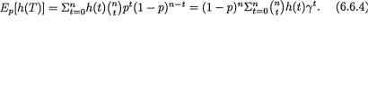
Example 6.6.3 Let X1, ..., Xn be iid Bernoulli(p), 0 < p < 1. We already know that  is a sufficient statistic for p. Let us verify that T is complete too. Since T is distributed as Binomial(n, p), the pmf induced by T is given by g(t; p) =
  pt(1 - p)n-t, t T = {0, 1, ..., n}. Consider any real valued
function h(t) such that Ep[h(T)] = 0 for all 0 < p < 1. Now, let us focus on the possible values of h(t) for t = 0, 1, ..., n. With γ = p(1 - p)-1, we can write
From (6.6.4) we observe that Ep[h(T)] has been expressed as a polynomial of the nth degree in terms of the variable γ (0, ∞). A nth degree polynomials in ? may be equal to zero for at most n values of γ (0, ∞). If we are forced to assume that
then we conclude that  that is
  for all t = 0,
1, ..., n. In other words, h(t) ≡ 0 for all t = 0, 1, ..., n, proving the completeness of the sufficient statistic T. !
 is a sufficient statistic for
  = {1,
= {1,  happens to be the
 will be unable to generate all infinite power series in
  are
are  that is
  ,
,  ) =
) = 
 –
–  –
–  –
– 
6. Sufficiency, Completeness, and Ancillarity |
322 |
U, and hence by the Theorem 6.3.2, T itself is a minimal sufficient statistic for
θ. But recall that Eθ(Xn:1) = (1 + n-1)θ and Eθ[(n – 1)–1 ∑ni=1(Xi-Xn:1)] = θ for all θ > 0. Let us denote h(t) = (1 + n–1)–1xn:1 – (n – 1)–1  for all tT = (θ, ∞) × +, so that Eθ[h(T)] = Eθ[(1 + n–1)–1 Xn:1 – (n – 1)–1
 = 0 for all θ > 0. But obviously h(t) is not identically zero for all t T ≡ (θ, ∞) × +. Hence, the minimal sufficient statistic T can not be complete. !
In the Examples 6.6.5-6.6.6, one can easily find other nontrivial real valued functions h(t) such that Eθ[h(T)] ≡ 0 for all θ, but h(t) is not identically zero. We leave these as exercises.
Theorem 6.6.1 Suppose that a statistic T = (T1, ..., Tk) is complete. Let U = (U1, ..., Uk) be another statistic with U = f(T) where g: T → U is one-to one. Then, U is complete.
Proof For simplicity, let us pretend that T, U have continuous distributions and that T, U and θ are all real valued. Let the pdf of T be denoted by g(t; θ). Since f(.) is one-to-one, we can write:
Now, assume that U is not complete. Then, there is a function a(U) such that
Eθ[a(U)] ≡ 0 but Pθ{u : a(u) ≠ 0} > 0 for all θ Θ. From (6.6.7) we can then claim that Eθ[h(T)] ≡ 0 for all θ Θ where h ≡ aof stands for the composition
mapping. But, this function h(.) is non-zero with positive probability which contradicts the assumed completeness property of T. !
Now, we state a remarkably general result (Theorem 6.6.2) in the case of the exponential family of distributions. One may refer to Lehmann (1986, pp. 142-143) for a proof of this result.
Theorem 6.6.2 (Completeness of the Minimal Sufficient Statistic in the Exponential Family) Suppose that X1, ..., Xn are iid with the common pmf or the pdf belonging to the k-parameter exponential family defined by
with some appropriate forms for p(x) ≥ 0, q(θ) ≥ 0, θi and Ri(x), i = 1, ..., k. Suppose that the regulatory conditions stated in (3.8.5) hold. Denote

6. Sufficiency, Completeness, and Ancillarity |
323 |
the statistic  Rj(Xi), j = 1, ..., k. Then, the (jointly) minimal sufficient statistic T = (T1, ..., Tk) for θ is complete.
Theorem 6.6.2 will sometimes provide an easy route to claim the completeness of a sufficient statistic for θ as long as f(x; θ) is given by (6.6.9) and the parameter space Θ( k)
includes a k-dimensional rectangle.
Example 6.6.7 Let X1, ..., Xn be iid N(µ, σ2) with (µ, σ) Θ = × + where µ and σ are both assumed unknown. The pdf of N(µ, σ2) has the form
given in (6.6.9) where k = 2, θ = (θ1, θ2) with θ1 = µ/σ2, θ2 = 1/σ2, R1(x) = x, R2(x) = x2, so that the minimal sufficient statistic is T = T(X) = (T1(X), T2(X))
where  and
and  . In view of the Theorem 6.6.2, the statistic T(X) is complete. !
Example 6.6.8 Let X1, ..., Xn be iid Gamma(α, β) so that f(x; α, β) = {βαΓ(α)}-1 exp(–x/β)xα-1 with (α, β) + × +, x + where the parameters
α and β are both assumed unknown. This pdf has the form given in (6.6.9)
where k = 2, θ = (θ1, θ2) with θ1 = 1/β, θ2 = α, R1(x) = –x, R2(x) = log(x), so that the sufficient statistic is T(X) = (T1(X), T2(X)) where 
and  . In view of the Theorem 6.6.2, the statistic T is complete. !
Example 6.6.9 In the Example 6.6.7, if µ is assumed unknown, but σ is known, then  or equivalently
  is a complete sufficient statistic for µ. In that same example, if µ is known, but σ is unknown, then
  is a complete sufficient statistic for σ. In the Ex-
ample 6.6.8, if α is unknown, but β is known, then  is a complete sufficient statistic for α. In this case if α is known, but β is unknown, then
  or
or  equivalently is a complete sufficient statistic for β. These results follow immediately from the Theorem 6.6.2. !
Example 6.6.10 (Example 6.6.4 Continued) Suppose that we have X1, ..., Xn iid Poisson(λ) where λ(> 0) is the unknown parameter. The common pmf f(x; λ) = e–λλx/x! with χ = {0, 1, 2, ...}, θ = log(λ) has the same representation given in (6.6.9) where k = 1, p(x) = (x!)-1, q(λ) = exp{e–θ} and R(x) = x. Hence, in view of the Theorem 6.6.2, the sufficient statistic  is then complete. !
Theorem 6.6.2 covers a lot of ground by helping to prove the completeness property of sufficient statistics. But it fails to reach out to non-exponential family members. The case in point will become clear from the Example 6.6.11.
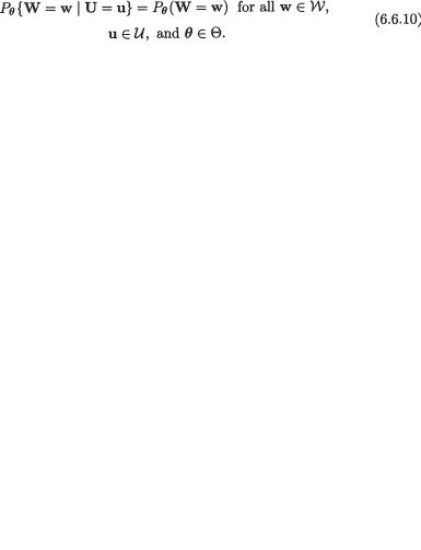
6. Sufficiency, Completeness, and Ancillarity |
324 |
Example 6.6.11 (Example 6.2.13 Continued) Suppose that X1, ..., Xn are iid Uniform(0, θ), θ(> 0) being the unknown parameter. We know that T(X) =
Xn:n is a minimal sufficient statistic for θ and the pdf of T is given by f(t; θ) = ntn-1θ–n I(0 < t < θ) which does not belong to the exponential family defined by
(6.6.9) with k = 1. But, we show directly that T is complete. Let h(t), 0 < t < θ, be any arbitrary real valued function such that Eθ[h(T)] = 0 for all θ > 0 and we can write
which proves that h(θ) ≡ 0 for all θ > 0. We have now shown that the minimal sufficient statistic T is complete. See (1.6.16)-(1.6.17) for the rules on differentiating an integral. !
6.6.2Basu’s Theorem
Suppose that X = (X1, ..., Xn) has the likelihood function L which depends on some unknown parameter ! and the observed value x. It is not essential to assume that X1, ..., Xn are iid in the present setup. Consider now two statistics U = U(X) and W = W(X). In general, showing that the two statistics U and W are independent is a fairly tedious process. Usually, one first finds the joint pmf or pdf of (U, W) and then shows that it can be factored into the two marginal pmf’s or pdf’s of U and W.
The following theorem, known as Basu’s Theorem, provides a scenario under which we can prove independence of two appropriate statistics painlessly. Basu (1955a) came up with this elegant result which we state here under full generality.
Theorem 6.6.3 (Basu’s Theorem) Suppose that we have two vector valued statistics, U = U(X) which is complete sufficient for θ and W = W(X) which is ancillary for θ. Then, U and W are independently distributed.
Proof For simplicity, we supply a proof only in the discrete case. The proof in the continuous situation is similar. Suppose that the domain spaces for U and W are respectively denoted by U and W.
In order to prove that U and W are independently distributed, we need to show that
Now, for w W, let us denote Pθ(W = W) = h(W). Obviously h(W) is free from θ since W’s distribution does not involve the parameter θ.

6. Sufficiency, Completeness, and Ancillarity |
325 |
But, observe that Pθ{W = w | U = u} must be free from θ since U is a sufficient statistic for θ. So, let us write g(u) = Pθ{W = w | U = u}. Now, Eθ[g(U)] = Pθ(W = w) which we had denoted earlier by h(w), and this is free from θ. Hence, we have verified that {g(U) - h(w)} is a genuine statistic.
Now, we note that Eθ[g(U) – h(w)] ≡ 0 for all θ Θ and use the fact that the statistic U is complete too. Thus, by the Definition 6.6.3 we must have g(u) – h(w) = 0 w.p.1, that is, g(u) ≡ h(w) for all w W, u U. In other words, we have shown the validity of (6.6.10). !
Example 6.6.12 Let X1, ..., Xn be iid N(µ, σ2) with n ≥ 2, (µ, σ) × + where µ is unknown, but σ is known. Let U =  which is complete sufficient
statistic for µ. Observe that W = S2 is an ancillary statistic for µ. The fact that W is ancillary can be claimed from its explicit distribution or by appealing to the location family of distributions. Now, by Basu’s Theorem, the two statistics  and S2 are then independently distributed. The Theorem 4.4.2 showed this via Helmert transformation. !
Example 6.6.13 (Example 6.6.12 Continued) Let V = Xn:n - Xn:1, the sample range. Then,  and S/V are independently distributed. Also,
  and (Xn:n –
  ) are independent. In the same spirit, and (Xn:1 –
  )2 are independent. Is
  independent of | Xn:n –
  | /S? The ancillarity of the corresponding statistics can be verified by appealing to the location family of distributions. We leave out the details as exercises. !
Example 6.6.14 Let X1, ..., Xn be iid N(µ, σ2) with n ≥ 2, (µ, σ) × + where σ is unknown, but µ is known. Let U2 =  which is a
complete sufficient statistic for σ2. Observe that W = (X1 –  )/U is ancillary for σ. Immediately we can claim that
  and W are independently distributed. Also,
  and (Xn:1 –
  )/S are independent where S2 is the customary sample variance. Here, ancillarity of the corresponding statistics can be verified by appealing to the scale family of distributions. We leave out the details as exercises. !
In the N(µ, s2) case with µ, s both unknown, Basu’s Theorem can
be used to show that  and S2 are independent. See the Example 6.6.15. Compare its elegance with the brute-force approach given in the Example 4.4.9 via Helmert transformations.
Example 6.6.15 Suppose that X1, ..., Xn are iid N(µ, σ2) with n ≥ 2, (µ, σ) × + where µ and σ are both assumed unknown. Let us see how we can apply Basu’s Theorem to show that  and S2 are independently distributed. This clever application was originated by D. Basu. Let us have
6. Sufficiency, Completeness, and Ancillarity |
326 |
any two sets A , B + and we wish to verify that
We now work with a fixed but otherwise arbitrary value σ = σ0(> 0). In this situation, we may pretend that µ is really the only unknown parameter so that we are thrown back to the setup considered in the Example 6.6.12, and hence claim that  is complete sufficient for µ and S2 is ancillary for µ. Thus, having fixed σ = σ0, using Basu’s Theorem we claim that
  and S2 will be independently distributed. That is, for all µ and fixed σ0(> 0), we have so far shown that
But, then (6.6.12) holds for any fixed value σ0 +. That is, we can claim the validity of (6.6.12) for all (µ, σ0) × +. There is no difference between what we have shown and what we started out to prove in (6.6.11). Hence, (6.6.11) holds. !
From the Example 6.6.15, the reader may think that we used the sufficiency property of  and ancillarity property of S2. But if µ, s are both unknown, then certainly
  is not sufficient and S2 is not ancillary. So, one may think that the previous proof must be wrong. But, note that we used the following two facts only: when σ = σ0 is fixed but arbitrary,
  is sufficient and S2 is ancillary.
Example 6.6.16 (Example 6.6.15 Continued) In the Example 6.6.15, the statistic U = ( , S2) is complete sufficient for θ = (µ, σ2) while W = (X1 – X2)/S is a statistic whose distribution does not depend upon θ. Here, we may use the characteristics of a location-scale family. To check directly that W has a distribution which is free from θ, one may pursue as follows: Let Yi = (Xi – µ)/σ which are iid standard normal, i = 1, ..., n, and then note that the statistic W can also be expressed as (Y1 - Y2)/S* where S*2 = (n – 1)-1
 with
with  . The statistics U and W are independent by virtue of Basu’s Theorem. In this deliberation, the ancillary statistic W can be vector valued too. For example, with n ≥ 3, suppose that we define
W* = ({X1 – X2}/S, {X2 – X3}/|X1 + X2 – 2X3|). As before, we can rewrite W* as ({Y1 – Y2}/S*, {Y2 – Y3}/|Y1 + Y2 – 2Y3|) where we recall that the Y’s are iid standard normal, and hence W* is ancillary for θ. Hence, U and W*
are independent by virtue of Basu’s Theorem. !

6. Sufficiency, Completeness, and Ancillarity |
327 |
In the Examples 6.6.12-6.6.15, the arguments revolved around sufficiency and completeness to come face to face with the result that  and S2 are independent. A reader may get the wrong impression that the completeness property is essential to claim that
  and S2 are independent. But, note that (
 , S2) is not a complete statistic when we have random samples from N(θ, θ) or N(θ, θ2) population, with θ > 0. Yet it is true that
  and S2 are independent in such situations. Refer to the Example 4.4.9.
Example 6.6.17 (Example 6.6.15 Continued) Suppose that X1, ..., Xn are iid N(µ, σ2) with (µ, σ) × + where µ and σ are both assumed unknown. By Basu’s Theorem, one can immediately claim that the statistic ( , S2) and (X1 –
  )/(Xn:n – Xn:1) are independent. !
Example 6.6.18 (Example 6.6.11 Continued) Suppose that X1, ..., Xn are iid Uniform(0, θ) with n ≥ 2, θ(> 0) being the unknown parameter. We know
that U = Xn:n is a complete sufficient statistic for θ. Let W = Xn:1/Xn:n which is ancillary for θ. Hence, by Basu’s Theorem, Xn:n and Xn:1/Xn:n are independently distributed. Also, Xn:n and  /S are independent, since
  /S is ancillary
for θ where S2 stands for the sample variance. Using a similar argument, one
can also claim that (Xn:n – Xn:1/S and Xn:n are independent. One may look at the scale family of distributions to verify the ancillarity property of the appropri-
ate statistics. !
Remark 6.6.1 We add that a kind of the converse of Basu’s Theorem was proved later in Basu (1958). Further details are omitted for brevity.
6.7Exercises and Complements
6.2.1Suppose that X1, X2 are iid Geometric(p), that is the common pmf is given by f(x;p) = p(1 – p)x, x = 0, 1, 2, ... where 0 < p < 1 is the unknown parameter. By means of the conditional distribution approach, show that X1 + X2 is sufficient for p.
6.2.2Suppose that X1, ..., Xm are iid Bernoulli(p), Y1, ...., Yn are iid Bernoulli(q), and that the X’s are independent of the Y’s where 0 < p < 1 is the unknown parameter with q = 1 - p. By means of the conditional distribu-
tion approach, show that  is sufficient for p. {Hint: Instead of looking at the data (X1, ..., Xm, Y1, ...., Yn), can one justify looking at (X1, ..., Xm, 1 - Y1, ...., 1 - Yn)?}
6. Sufficiency, Completeness, and Ancillarity |
328 |
6.2.3Suppose that X is distributed as N(0, σ2) where 0 < σ < ∞ is the unknown parameter. Along the lines of the Example 6.2.3, by means of the conditional distribution approach, show that the statistic | X | is sufficient for
σ2.
6.2.4Suppose that X is N(θ, 1) where –∞ < θ < ∞ is the unknown param-
eter. By means of the conditional distribution approach, show that | X | can not be sufficient for θ.
6.2.5(Exercise 6.2.2 Continued) Suppose that m = 2, n = 3. By means of
the conditional distribution approach, show that X1 + Y1Y2 can not be sufficient for p.
6.2.6Suppose that X1, ..., Xm are distributed as iid Poisson(λ), Y1, ..., Yn are iid Poisson(2λ), and that the X’s are independent of the Y’s where 0 < λ < ∞ is the unknown parameter. By means of the conditional distribution ap-
proach, show that  is sufficient for ?.
6.2.7(Exercise 6.2.6 Continued) Suppose that m = 4, n = 5. Show that X1
+Y1 can not be sufficient for λ.
6.2.9(Example 6.2.5 Continued) Let X1, ..., X4 be iid Bernoulli(p) where 0 < p < 1 is the unknown parameter. Consider the statistic U = X1(X3 + X4) + X2. By means of the conditional distribution approach, show that the statistic U is not sufficient for p.
6.2.10Let X1, ..., Xn be iid N(µ, σ2) where –∞ < µ < ∞, 0 < σ < ∞. Use the Neyman Factorization Theorem to show that
(i) |
is sufficient for µ if σ is known; |
(ii) |
is sufficient for σ if µ is known. |
6.2.11Let X1, ..., Xn be iid having the common pdf σ–1 exp{–(x – µ)/σ}I(x
>µ) where –∞ < µ < ∞, 0 < σ < ∞. Use the Neyman Factorization Theorem to show that
(i) |
Xn:1, the smallest order statistic, is sufficient for µ if σ is known; |
(ii) |
is sufficient for σ if µ is known; |
(iii) |
is jointly sufficient for (µ, σ) if both |
|
parameters are unknown. |
6.2.12 Let X1, ..., Xn be iid having the Beta(α, β) distribution with the parameters α and β, so that the common pdf is given by
6. Sufficiency, Completeness, and Ancillarity |
329 |
where b(α, β) = Γ(α)Γ(β){Γ(α + β)}–1. Refer to (1.7.35) as needed. Use the Neyman Factorization Theorem to show that
(i) |
is sufficient for α if β is known; |
(ii) |
is sufficient for β if α is known; |
(iii) |
is jointly sufficient for (α, β) if both |
|
parameters are unknown. |
6.2.13Suppose that X1, ..., Xn are iid with the Uniform distribution on the interval (θ - ½, θ + ½), that is the common pdf is given by f(x; θ) = I(θ – ½
<x < θ + ½) where θ(> 0) is the unknown parameter. Show that (Xn:1, Xn:n) is jointly sufficient for θ.
6.2.14Solve the Examples 6.2.8-6.2.11 by applying the Theorem 6.2.2 based on the exponential family.
6.2.15Prove the Theorem 6.2.2 using the Neyman Fctorization Theorem.
6.2.16Suppose that X1, ..., Xn are iid with the Rayleigh distribution, that is the common pdf is
where θ(> 0) is the unknown parameter. Show that  is sufficient for
θ.
6.2.17 Suppose that X1, ..., Xn are iid with the Weibull distribution, that is the common pdf is
where α(> 0) is the unknown parameter, but β(> 0) is assumed known that  is sufficient for α.
6.3.1(Exercise 6.2.10 Continued) Let X1, ..., Xn be iid N(µ, σ2) where –∞
<µ < ∞, 0 < σ < ∞. Show that
(i) is minimal sufficient for µ if σ is known; (ii) is minimal sufficient for σ if µ is known.
6.3.2 (Exercise 6.2.11 Continued) Let X1, ..., Xn be iid having the common pdf σ–1 exp{–(x – µ)/σ}I(x > µ) where –∞ < µ < ∞, 0 < σ < ∞. Show that
(i) Xn:1, the smallest order statistic, is minimal sufficient for µ if
σis known;
(ii) |
is minimal sufficient for s if µ is known; |
(iii) |
is minimal sufficient for (µ, σ) if both |
|
parameters are unknown. |
6. Sufficiency, Completeness, and Ancillarity |
330 |
6.3.3Solve the Exercises 6.2.5-6.2.8 along the lines of the Examples 6.3.2 and 6.3.5.
6.3.4Show that the pmf or pdf corresponding to the distributions such as Binomial(n, p), Poisson(λ), Gamma(α, β), N(µ, σ2), Beta(α, β) belong to the exponential family defined in (6.3.5) when
(i) 0 < p < 1 is unknown; (ii) λ + is unknown;
(iii) µ is unknown but σ + is known; (iv) σ + is unknown but µ is known; (v) µ and σ + are both unknown; (vi) α + is known but β + is unknown; (vii) α +, β + are both unknown.
In each case, obtain the minimal sufficient statistic(s) for the associated unknown parameter(s).
6.3.5 (Exercise 6.2.1 Continued) Let X1, ..., Xn be Geometric(p), that is the common pmf is given by f(x;p) = p(1 - p)x, x = 0, 1, 2, ... where 0 < p < 1 is the unknown parameter. Show that this pmf belongs to the exponential family defined in (6.3.5). Hence, show that  is minimal sufficient for p.
6.3.6. Show that the common pdf given in the Exercises 6.2.16-6.2.17 respectively belongs to the exponential family.
6.3.7Suppose that X1, ..., Xn are iid with the Uniform distribution on the interval (θ – ½, θ + ½), that is the common pdf is given by f(x;θ) = I(θ – ½ <
x < θ + ½) where θ(> 0) is the unknown parameter. Show that (Xn:1, Xn:n) is jointly minimal sufficient for θ.
6.3.8Let X1, ..., Xn be iid N(θ, θ2) where 0 < θ < ∞ is the unknown parameter. Derive the minimal sufficient statistic for ∞. Does the common pdf belong to the exponential family (6.3.5)? {Hint: If it does belong to the
exponential family, it should be a 2-parameter family, but it is not so. Does the parameter space include a 2-dimensional rectangle?}
6.3.9Let X1, ..., Xn be iid N(θ, θ) where 0 < θ < ∞ is the unknown parameter. Derive the minimal sufficient statistic for θ. Does the common pdf belong to the exponential family (6.3.5)? {Hint: If it does belong to the exponen-
tial family, it should be a 2-parameter family, but it is not so. Does the parameter space include a 2-dimensional rectangle?}
6.3.10Let X1, ..., Xn be iid having a negative exponential distribution with the common pdf θ–1 exp{–(x – θ)/θ}I(x > θ) where 0 < θ < ∞ is the unknown parameter. Derive the minimal sufficient statistics for θ. Does the common pdf belong to the exponential family (6.3.5)? {Hint: If it does
6. Sufficiency, Completeness, and Ancillarity |
331 |
belong to the exponential family, it should be a 2-parameter family, but it is not so. Does the parameter space include a 2-dimensional rectangle?}
6.3.11Let X1, ..., Xn be iid having a negative exponential distribution with the common pdf θ–2 exp{–(x – θ)/θ2}I(x > θ) where 0 < θ < ∞ is the unknown parameter. Derive the minimal sufficient statistics for θ. Does the common pdf belong to the exponential family (6.3.5)? {Hint: If it does belong to the
exponential family, it should be a 2-parameter family, but it is not so. Does the parameter space include a 2-dimensional rectangle?}
6.3.12Let X1, ..., Xn be iid having the common Uniform distribution on the interval (–θ, θ) where 0 < θ < ∞ is the unknown parameter. Derive the minimal sufficient statistic for θ.
6.3.13Let X1, ..., Xm be iid N(µ1, σ2), Y1, ..., Yn be iid N(µ2, σ2), and also let the X’s be independent of the Y’s where –∞ < µ1, µ2 < ∞, 0 < σ < ∞ are the unknown parameters. Derive the minimal sufficient statistics for (µ1, µ2, σ2).
6.3.14(Exercise 6.3.13 Continued) Let X1, ..., Xm be iid N(µ1, σ2), Y1, ..., Yn be iid N(µ2, kσ2), and also let the X’s be independent of the Y’s where –∞
<µ1, µ2 < ∞, 0 < σ < ∞ are the unknown parameters. Assume that the number k (> 0) is known. Derive the minimal sufficient statistic for (µ1, µ2, σ2).
6.3.15Let X1, ..., Xm be iid Gamma(α, β), Y1, ..., Yn be iid Gamma(α, kβ), and also let the X’s be independent of the Y’s with 0 < α, β < ∞ where β is the
only unknown parameter. Assume that the number k (> 0) is known. Derive the minimal sufficient statistic for β.
6.3.16(Exercise 6.2.12 Continued) Let X1, ..., Xn be iid having a Beta distribution with its parameters α = β = θ where θ (> 0) is unknown. Derive the minimal sufficient statistic for θ.
6.3.17Let X1, ..., Xm be iid N(µ, σ2), Y1, ..., Yn be iid N(0, σ2), and also let the X’s be independent of the Y’s where –∞ < µ < ∞, 0 < σ < ∞ are the unknown parameters. Derive the minimal sufficient statistics for (µ, σ2).
6.3.18Let X1, ..., Xm be iid N(µ, σ2), Y1, ..., Yn be iid N(0, kσ2), and also let the X’s be independent of the Y’s where –∞ < µ < ∞, 0 < σ < ∞ are the
unknown parameters. Assume that the number k (> 0) is known. Derive the minimal sufficient statistics for (µ, σ2).
6.3.19Suppose that X1, ..., Xn are iid with the common pdf given by one of the following:

6. Sufficiency, Completeness, and Ancillarity |
332 |
(i) f(x; θ) = exp(–(x – θ)}/[1 + exp{–(x – θ)}]2, x , θ , which is called the logistic distribution;
(ii) f(x; θ) = 1/π{1 + (x – θ)2}–1, x , ? ; (iii) f(x; θ) = ½ exp{– | x – θ |}, x , ? .
In each case, show that the order statistics (Xn:1, ..., Xn:n) is minimal sufficient for the unknown location parameter θ. That is, we do not achieve any significant reduction of the original data X = (X1, ..., Xn). {Hint: Part (i) is proved in Lehmann (1983, p. 43). Parts (ii) and (iii) can be handled similarly.}
6.4.1 Let X1, ..., Xn be iid Bernoulli(p) where 0 < p < 1 is the unknown parameter. Evaluate IX(p), the information content in the whole data X = (X1,
..., Xn). Compare IX(p) with  . Can the Theorem 6.4.2 be used here to claim that
  is sufficient for p?
6.4.2 (Exercise 6.4.1 Continued) Let X1, ..., Xn be iid Bernoulli(p) where 0
< p < 1 is the unknown parameter, n ≥ 3. Let T = X1 + X2, U = X1 + X2 + 2X3. Compare IX(p) with IT(p) and IU(p). Can T be sufficient for p? Can U be
sufficient for p? {Hint: Try to exploit the Theorem 6.4.2}
6.4.3Verify the results given in equations (6.4.9) and (6.4.11).
6.4.4(Exercise 6.2.1 Continued) Let X1, X2, be iid Geometric(p) where 0
<p < 1 is the unknown parameter. Let X = (X1, X2), and T = X1 + X2 which is sufficient for p. Evaluate IX(p) and IT(p), and then compare these two information contents.
6.4.5(Exercise 6.2.10 Continued) In a N(µ, σ2) distribution where –∞ < µ
<∞, 0 < σ < ∞, suppose that only µ is known. Show that IU2(s2) > IS2(s2)
≥2.where U
Would it then be fair to say that there is no point in using the statistic S2 which making inferences about σ2 when µ is assumed known?
6.4.6 (Exercise 6.2.11 Continued) In the two-parameter negative exponential distribution, if only µ is known, show that IV(σ) > IT(σ) where V = n– 1  and T = (n - 1)-1
  , n ≥ 2. Would it then be fair to say that there is no point in using the statistic T while making inferences about σ when µ is assumed known?
6.4.7(Exercise 6.3.17 Continued) Suppose that we have X1, ..., Xm are iid N(µ, σ2), Y1, ..., Yn are iid N(0, σ2), the X’s are independent of the Y’s where
–∞ < µ < ∞, 0 < σ < ∞ are the unknown parameters. Suppose that T = T(X, Y) is the minimal sufficient statistic for θ = (µ, σ2). Evaluate the expressions
of the information matrices IX,Y(θ) and IT(θ), and then compare these two information contents.
6.4.8(Example 6.2.5 Continued) Consider the statistics X1X2 and U.
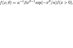
6. Sufficiency, Completeness, and Ancillarity |
333 |
Find the pmf of X1X2 and then using the fact that X1X2 is independent of X3, derive the pmf of U. Hence, find the expressions of IX(p), and 
IU(p) where X = (X1, X2, X3). Show that IU(p) <  < IX(p). This shows that U or (X1X2, X3) can not be sufficient for p.
6.4.9 (Exercise 6.2.16 Continued) Suppose that X1, ..., Xn are iid with the Rayleigh distribution, that is the common pdf is
where θ(> 0) is the unknown parameter. Denote the statistic  . Evaluate IX(θ) and IT(θ). Are these two information contents the same? What conclusions can one draw from this comparison?
6.4.10 (Exercise 6.2.17 Continued) Suppose that X1, ..., Xn are iid with the Weibull distribution, that is the common pdf is
where α (> 0) is the unknown parameter, but β(> 0) is assumed known. Denote the statistic T=Σin=1X2i. Evaluate IX(θ) and IT(θ). Are these two information contents the same? What conclusions can one draw from this comparison?
6.4.11Prove the Theorem 6.4.3. {Hint: One may proceed along the lines of the proof given in the case of the Theorem 6.4.1.}
6.4.12Prove the Theorem 6.4.4 when
(i) X, θ are both vector valued, but X has a continuous distribution; (ii) X, θ are both real valued, but X has a discrete distribution.
6.4.13 (Exercise 6.3.8 Continued) Let X1, ..., Xn be iid N(θ, θ2) where 0 < θ < ∞ is the unknown parameter. Evaluate IX(θ) and  , and compare these two quantities. Is it possible to claim that
  is sufficient for θ?
6.4.14 (Exercise 6.3.9 Continued) Let X1, ..., Xn be iid N(θ, θ) where 0 < θ < ∞ is the unknown parameter. Evaluate IX(θ) and  , and compare these two quantities. Is it possible to claim that
  is sufficient for θ?
6.4.15 (Proof of the Theorem 6.4.2) Let θ be a real valued parameter. Suppose that X is the whole data and T = T(X) is some statistic. Then, show that IX(θ) ≥ IT(θ) for all θ Θ. Also verify that the two information measures match with each other for all θ if and only if T is a sufficient statistic for θ. {Hint: This interesting idea was included in a recent personal
6. Sufficiency, Completeness, and Ancillarity |
334 |
communication from C. R. Rao. Note that the likelihood function f(x; θ) can be written as g(t; θ)h(X | T = t; θ) where g(t; θ) is the pdf or pmf of T and h(x | T = t; θ) is the conditional pdf or pmf of X given that T = t. From this equality, first derive the identity: IX(θ) = IT(θ) + IX|T(θ) for all θ Θ. This
implies that IX(θ) ≥ IT(θ) for all θ Θ. One will have IX(θ) = IT(θ) if and only if IX|T(θ) = 0, that is h(x | T = t;θ) must be free from θ. It then follows from
the definition of sufficiency that T is sufficient for θ.}
6.4.16Suppose that X1, X2 are iid N(θ, 1) where the unknown parameter θ
. ‘We know that T = X1 + X2 is sufficient for θ and also that IT(θ) = 2. Next, consider a statistic Up = X1 + pX2 where p is a known positive number.
(i) Show that IUp(θ) = (1 + p)2/(1 + p2); (ii) Show that 1 < IUp(θ) ≤ 2 for all p(> 0); (iii) Show that IUp(θ) = 2 if and only if p = 1;
(iv) An expression such as IUp(θ)/IT(θ) may be used to quantify the extent of non-sufficiency or the fraction of the lost information due to
using Up instead of utilizing the sufficient statistic T. Analytically, study the behavior of IUp(θ)/IT(θ) as a function of p(> 0);
(v) Evaluate IUp(θ)/IT(θ) for p = .90, .95, .99, 1.01, 1.05, 1.1. Is Up too non-sufficient for θ in practice when p = .90, .95, .99, 1.01?
(vi) In practice, if an experimenter is willing to accept at the most 1% lost information compared with the full information IT(θ), find the range of values of p for which the non-sufficient statistic Up will attain the goal.
{Note: This exercise exploits much of what has been learned conceptually from the Theorem 6.4.2.}
6.5.1(Example 6.5.2 Continued) Find the pdf of U3 defined in (6.5.1). Hence, show that T3 is ancillary for θ.
6.5.2(Example 6.5.3 Continued) Show that T3 is ancillary for λ.
6.5.3(Example 6.5.4 Continued) Show that T = (T1, T2) is distributed as N2(0, 0, 2, 6, 0). Are T1, T2 independent?
6.5.4(Example 6.5.5 Continued) Show that T is ancillary for θ.
6.5.5(Exercise 6.3.7 Continued) Let X1, ..., Xn be iid having the common Uniform distribution on the interval (θ – ½, θ + ½) where –∞ < θ < ∞ is the unknown parameter. Show that Xn:n – Xn:1 is an ancillary statistic for θ.
6. Sufficiency, Completeness, and Ancillarity |
335 |
6.5.6 (Exercise 6.3.12 Continued) Let X1, ..., Xn be iid having the common Uniform distribution on the interval (–θ, θ) where 0 < θ < ∞ is the unknown parameter. Show that Xn:n/Xn:1 is an ancillary statistic for θ. Also show that Xn:n/(Xn:n – Xn:1) is an ancillary statistic for θ.
6.5.7 (Curved Exponential Family) Suppose that (X, Y) has a particular curved exponential family of distributions with the joint pdf given by
where θ(> 0) is the unknown parameter. This distribution was discussed by Fisher (1934, 1956) in the context of the famous “Nile” example. Denote U = XY, V = X/Y. Show that U is ancillary for θ, but (U, V) is minimal sufficient for θ, whereas V by itself is not sufficient for θ. {Hint: The answers to the Exercise 4.4.10 would help in this problem.}
6.5.8Show that the families F1, F2, F3 defined via (6.5.7) include only genuine pdf’s.
6.5.9(Exercise 6.3.8 Continued) Let X1, ..., Xn be iid N(θ, θ2) where 0 < θ
<∞ is the unknown parameter. Construct several ancillary statistics for θ. Does the common pdf belong to one of the special families defined via (6.5.7)?
6.5.10(Exercise 6.3.9 Continued) Let X1, ..., Xn be iid N(θ, θ) where 0 < θ < 8 is the unknown parameter. Construct several ancillary statistics for θ. Does the common pdf belong to one of the special families defined via (6.5.7)?
6.5.11(Exercise 6.3.10 Continued) Let X1, ..., Xn be iid having the common pdf θ–1 exp{ – (x – θ)/θ}I(x > θ) where 0 < θ < 8 is the unknown parameter. Construct several ancillary statistics for θ. Does the common pdf belong to one of the special families defined via (6.5.7)?
6.5.12(Exercise 6.3.11 Continued) Let X1, ..., Xn be iid having the common pdf θ–2 exp{ – (x – θ)/θ2}I(x > θ) where 0 < θ < ∞ is the unknown parameter. Construct several ancillary statistics for θ. Does the common pdf belong to one of the special families defined via (6.5.7)?
6.5.13Use the Definition 6.4.1 of the information and the pdf from (6.5.4)
to derive directly the expression for IX,Y(ρ). {Hint: Take the log of the pdf from (6.5.4). Then take the partial derivative of this with respect to ?. Next,
square this partial derivative and take its expectation.}
6.5.14 Suppose that (X, Y) is distributed as N2(0, 0, σ2, σ2, ρ) where -1 < ρ < 1 is the unknown parameter while 0 < σ (≠ 1) < ∞ is assumed known. Evaluate the expression for the information matrix IX,Y(ρ) along
6. Sufficiency, Completeness, and Ancillarity |
336 |
the lines of the Example 6.5.8. Next, along the lines of the Example 6.5.11, recover the lost information in X by means of conditioning on the ancillary statistic Y.
6.5.15 (Example 6.5.8 Continued) Suppose that (X, Y) is distributed as N2(0, 0, σ2, σ2, ρ) where θ = (σ2, ρ) with the unknown parameters σ2, ρ where 0 < σ < ∞, –1 < ρ < 1. Evaluate the expression for the information
matrix IX,Y(θ). {Hint: Does working with U = X + Y, V = X - Y help in the derivation?}
6.5.16 Suppose that X′ = (X1, ..., Xp) where X is distributed as multivariate
normal Np (0, σ2[(1 – ρ)Ip×p + ρ11′]) with 1′ = (1, 1, ....1), σ + and – (p – 1)–1 < ρ < 1. We assume that θ = (σ2, ρ) where σ2, ρ are the unknown
parameters, 0 < σ < ∞, –1 < ρ < 1. Evaluate the expression for the information matrix IX(θ). {Hint: Try the Helmert transformation from the Example 2.4.9 on X to generate p independent normal variables each with zero mean, and variances depending on both σ2 and ρ, while (p - 1) of these variances are all equal but different from the pth one. Is it then possible to use the Theorem 6.4.3?}
6.5.17 (Example 6.5.8 Continued) Suppose that (X, Y) is distributed as N2(0, 0, 1, 1, ρ) where ρ is the unknown parameter, –1 < ρ < 1. Start with the pdf of (X, Y) and then directly apply the equivalent formula from the equation (6.4.9) for the evaluation of the expression of IX,Y(ρ).
6.6.1Suppose that X1, X2 are iid Poisson(λ) where λ(> 0) is the unknown parameter. Consider the family of distributions induced by the statistic T = (X1, X2). Is this family, indexed by λ, complete?
6.6.2(Exercise 6.3.5 Continued) Let X1, ..., Xn be iid Geometric(p), that is the common pmf is given by f(x; p) = p(1 - p)x, x = 0, 1, 2, ... where 0 < p <
1 is the unknown parameter. Is the statistic  complete sufficient for p? {Hint: Is it possible to use the Theorem 6.6.2 here?}
6.6.3Let X1, ..., Xn be iid N(θ, θ2) where 0 < θ < ∞ is the unknown parameter. Is the minimal sufficient statistic complete? Show that  and S2 are independent. {Hint: Can the Example 4.4.9 be used here to solve the second part?}
6.6.4Let X1, ..., Xn be iid N(θ, θ) where 0 < θ < ∞ is the unknown parameter. Is the minimal sufficient statistic complete? Show that  and S2 are independent. {Hint: Can the Example 4.4.9 be used here to solve the second part?}
6.6.5Let X1, ..., Xn be iid having a negative exponential distribution with the common pdf θ–1 exp{–(x – θ)/θ}I(x > θ) where 0 < θ < ∞ is the unknown parameter. Is the minimal sufficient statistic complete? Show

6. Sufficiency, Completeness, and Ancillarity |
337 |
that Xn:1 and  are independent. {Hint: Can the Example 4.4.12 be used here to solve the second part?}
6.6.6 Let X1, ..., Xn be iid having a negative exponential distribution with the common pdf θ–2exp{–(x – θ)/θ2}I(x > θ) where 0 < θ < ∞ is the unknown parameter. Is the minimal sufficient statistic complete? Show that Xn:1 and  are independent. {Hint: Can the Example 4.4.12 be used
here to solve the second part?}
6.6.7 Let X1, ..., Xn be iid having the common Uniform distribution on the interval (θ – ½, θ + ½) where –∞ < θ < ∞ is the unknown parameter. Is the minimal sufficient statistic T = (Xn:1, Xn:n) complete?
6.6.8 Let X1, ..., Xn be iid having the common Uniform distribution on the interval (–θ, θ) where 0 < θ < ∞ is the unknown parameter. Find the minimal sufficient statistic T for θ. Is the statistic T complete? {Hint: Use indicator functions appropriately so that the problem reduces to the common pdf’s of the random variables | Xi |, i = 1, ..., n.}
6.6.9 Let X1, ..., Xm be iid N(µ1, σ2), Y1, ..., Yn be iid N(µ2, σ2), the X’s are independent of the Y’s where –∞ < µ1, µ2 < ∞, 0 < σ < ∞ are all unknown
parameters. Is the minimal sufficient statistic for (µ1, µ2, σ2) complete? {Hint: Is it possible to use the Theorem 6.6.2 here?}
6.6.10(Exercise 6.3.13 Continued) Let X1, ..., Xm be iid N(µ1, σ2), Y1, ..., Yn be iid N(µ2, kσ2), the X’s be independent of the Y’s where –∞ < µ1, µ2 < ∞, 0 < σ < ∞ are all unknown parameters, but k (> 0) is known. Is the minimal
sufficient statistic for (µ1, µ2, σ2) complete? {Hint: Is it possible to use the Theorem 6.6.2 here?}
6.6.11(Exercise 6.3.15 Continued) Let X1, ..., Xm be iid Gamma(α, β), Y1,
..., Yn be iid Gamma(α, kβ), the X’s be independent of the Y’s, with 0 < α, β
<∞ where β is the only unknown parameter. Assume that the number k (> 0) is known. Is the minimal sufficient statistic for β complete? {Hint: Is it possible to use the Theorem 6.6.2 here?}
6.6.12(Exercise 6.3.16 Continued) Let X1, ..., Xn be iid having a Beta distribution with its parameters α = β = θ where θ (> 0) is unknown. Is the minimal sufficient statistic for θ complete? {Hint: Is it possible to use the Theorem 6.6.2 here?}
6.6.13(Exercise 6.6.9 Continued) Let the X’s be independent of the
Y’s, X1, ..., Xm be iid N(µ1, σ2), Y1, ..., Yn be iid N(µ2, σ2) where –∞ < µ1, µ2 < ∞, 0 < σ < ∞ are all unknown parameters. Use Basu’s Theorem
along the lines of the Example 6.6.15 to show that |
is distributed |

 . Is (
 –
– )
) ) – (
) – ( )}
)} ) – (
) – ( )}
)} . Is
. Is  .
. are independent.
 is complete if
  is complete if both
6. Sufficiency, Completeness, and Ancillarity |
339 |
{Hint: Part (ii) follows from the Theorem 6.6.2. One may look at Lehmann (1983, pp. 47-48) for details.}
6.6.19 Let X1, ..., X4 be iid N(µ, σ2) where –∞ < µ < ∞, 0 < σ < ∞ are both unknown parameters. Evaluate the expression for
where |
and S2 = 1/3 |
. {Note: Can Basu’s Theo- |
rem be used here?} |
|
|
This page intentionally left blank