


 ) where
 where
where  is unknown but fixed. In the Bayesian approach, the experimenter believes from the very beginning that the unknown parameter
 is assumed
  =
=  by
by  =
= 
 =
=  =
=  contained in the collected data as evidenced by the likelihood function
  =
= 478 10. Bayesian Methods
with what is known as a posterior distribution. All Bayesian inferences are then guided by this posterior distribution. This approach which originated from Bayes’s Theorem was due to Rev. Thomas Bayes (1783). A strong theoretical foundation evolved due to many fundamental contributions of de Finetti (1937), Savage (1954), and Jeffreys (1957), among others. The contributions of L. J. Savage were beautifully synthesized in Lindley (1980).
From the very beginning, R. A. Fisher was vehemently opposed to anything Bayesian. Illuminating accounts of Fisher’s philosophical arguments as well as his interactions with some of the key Bayesian researchers of his time can be found in the biography written by his daughter, Joan Fisher Box (1978). Some interesting exchanges between R. A. Fisher and H. Jeffreys as well as L. J. Savage are included in the edited volume of Bennett (1990). The articles of Buehler (1980), Lane (1980) and Wallace (1980) gave important perspectives on possible connections between Fisher’s fiducial inference and the Bayesian doctrine.
A branch of statistics referred to as “decision theory” provides a formal structure to find optimal decision rules whenever possible. Abraham Wald gave the foundation to this important area during the early to mid 1940’s. Wald’s (1950) book, Statistical Decision Functions, is considered a classic in this area. Berger (1985) treated modern decision theory with much emphasis on Bayesian arguments. Ferguson (1967), on the other hand, gave a more balanced view of the area. The titles on the cover of these two books clearly emphasize this distinction.
In Section 10.2, we give a formal discussion of the prior and posterior distributions. The Section 10.3 first introduces the concept of conjugate priors and then posterior distributions are derived in some standard cases when  has a conjugate prior. In this section, we also include an example where the assumed prior for
  is not chosen from a conjugate family. In Section 10.4, we develop the point estimation problems under the squared error loss function and introduce the Bayes estimator for
  . In the same vein, Section 10.5.1 develops interval estimation problems. These are customarily referred to as credible interval estimators of v. Section 10.5.2 highlights important conceptual differences between a credible interval estimator and a confidence interval estimator. Section 10.6 briefly touches upon the concept of a Bayes test of hypotheses whereas Section 10.7 gives some examples of Bayes estimation under non-conjugate priors.
We can not present a full-blown discussion of the Bayes theory at this level. It is our hope that the readers will get a taste of the underlying basic principles from a brief exposure to this otherwise vast area.
10. Bayesian Methods |
479 |
10.2 Prior and Posterior Distributions
The unknown parameter  itself is assumed to be a random variable having its pmf or pdf h(θ) on the space Θ. We say that h(θ) is the prior distribution of v. In this chapter, the parameter
  will represent a continuous real valued variable on Θ which will customarily be a subinterval of the real line . Thus we will commonly refer to h(θ) as the prior pdf of
  .
.
The evidence about v derived from the prior pdf is then combined with that obtained from the likelihood function by means of the Bayes’s Theorem (Theorem 1.4.3). Observe that the likelihood function is the conditional joint pmf or pdf of X = (X1, ..., Xn) given that  = θ. Suppose that the statistic T is (minimal) sufficient for θ in the likelihood function of the observed data X given that
  = θ. The (minimal) sufficient statistic T will be frequently real valued and we will work with its pmf or pdf g(t; θ), given that v = θ, with t Τ where T is an appropriate subset of .
For the uniformity of notation, however, we will treat T as a continuous variable and hence the associated probabilities and expectations will be written in the form of integrals over the space T. It should be understood that integrals will be interpreted as the appropriate sums when T is a discrete variable instead.
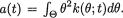
The joint pdf of T and v is then given by
The marginal pdf of T will be obtained by integrating the joint pdf from (10.2.1) with respect to θ. In other words, the marginal pdf of T can be written as
Thus, we can obtain the conditional pdf of v given that T = t as follows:
In passing, let us remark that the expression for k(θ; t) follows directly by applying the Bayes’s Theorem (Theorem 1.4.3). In the statement of the Bayes’s Theorem, simply replace  by k(θ; t),
h(θ), g(t; θ) and  respectively.
Definition 10.2.1 The conditional pdf k(θ; t) of  given that T = t is called the posterior distribution of
  .
.
480 10. Bayesian Methods
Under the Bayesian paradigm, after having the likelihood function and the prior, the posterior pdf k(θ;t) of v epitomizes how one combines the information about  obtained from two separate sources, the prior knowledge and the collected data. The tractability of the final analytical expression of k(θ;t) largely depends on how easy or difficult it is to obtain the expression of m(t). In some cases, the marginal distribution of T and the posterior distribution can be evaluated only numerically.
Example 10.2.1 Let X1, ..., Xn be iid Bernoulli(θ) given that v = θ where v is the unknown probability of success, 0 < v < 1. Given v = θ, the statistic
 is minimal sufficient for θ, and one has
where T = {0, 1, ..., n}. Now, suppose that the prior distribution of v on the space Θ = (0, 1) is taken to be Uniform(0, 1), that is h(θ) = I(0 < θ < 1). From (10.2.2), for t T, we then obtain the marginal pmf of T as follows:
Thus, for any fixed value t T, using (10.2.3) and (10.2.5), the posterior pdf of v given the data T = t can be expressed as
That is, the posterior distribution of the success probability v is described by the Beta(t + 1, n - t + 1) distribution. !
In principle, one may carry out similar analysis even if the unknown parameter v is vector valued. But, in order to keep the presentation simple, we do not include any such example here. Look at the Exercise 10.3.8 for a taste.
Example 10.2.2 (Example 10.2.1 Continued) Let X1, ..., X10 be iid Bernoulli(θ) given that  = θ where v is the unknown probability of success, 0 < v < 1. The statistic
  is minimal sufficient for θ given that
  = θ. Assume that the prior distribution of
  on the space Θ = (0, 1) is Uniform(0, 1). Suppose that we have observed the particular value T = 7,
10. Bayesian Methods |
481 |
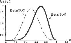
the number of successes out of ten Bernoulli trials. From (10.2.6) we know that the posterior pdf of the success probability  is that of the Beta(8, 4) distribution. This posterior density has been plotted as a solid curve in the Figure 10.2.1. This curve is skewed to the left. If we had observed the data T = 5 instead, then the posterior distribution of the success probability v will be described by the Beta(6, 6) distribution. This posterior density has been plotted as a dashed curve in the same Figure 10.2.1. This curve is symmetric about θ = .5. The Figure 10.2.1 clearly shows that under the same uniform prior
Figure 10.2.1. Posterior PDF’s of v Under Two Prior
Distributions of v When t = 7
regarding the success probability  but with different observed data, the shape of the posterior distribution changes one’s perception of what values of
  are more (or less) probable. !
10.3 The Conjugate Priors
If the prior h(θ) is such that the integral in the equation (10.2.2) can not be analytically found, then it will be nearly impossible to derive a clean expression for the posterior pdf k(θ; t). In the case of many likelihood functions, we may postulate a special type of prior h(θ) so that we can achieve technical simplicity.
Definition 10.3.1 Suppose that the prior pdf h(θ) for the unknown parameter v belongs to a particular family of distributions, P. Then, h(θ) is called a conjugate prior for  if and only if the posterior pdf k(θ; t) also belongs to the same family P.
What it means is this: if h(θ) is chosen, for example, from the family of
482 10. Bayesian Methods
beta distributions, then k(θ; t) must correspond to the pdf of an appropriate beta distribution. Similarly, for conjugacy, if h(θ) is chosen from the family of normal or gamma distributions, then k(θ; t) must correspond to the pdf of an appropriate normal or gamma distribution respectively. The property of conjugacy demands that h(θ) and k(θ; t) must belong to the same family of distributions.
Example 10.3.1 (Example 10.2.1 Continued) Suppose that we have the random variables X1, ..., Xn which are iid Bernoulli(θ) given that  = θ, where
  is the unknown probability of success, 0 <
  < 1. Given that
  = θ, the statistic
  is minimal sufficient for θ, and recall that one has
 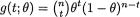 for t T = {0, 1, ..., n}.
In the expression for g(t; θ), carefully look at the part which depends on θ, namely θ t(1 - θ)n-t. It resembles a beta pdf without the normalizing constant. Hence, we suppose that the prior distribution of v on the space Θ = (0, 1) is Beta(α, β) where α (> 0) and β(> 0) are known numbers. From (10.2.2), for t T, we then obtain the marginal pmf of T as follows:
Now, using (10.2.3) and (10.3.1), the posterior pdf of v given the data T = t simplifies to
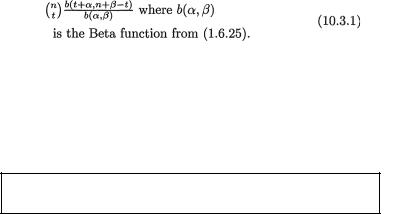
and fixed values t T. In other words, the posterior pdf of the success probability v is same as that for the Beta(t + α, n – t + β) distribution.
We started with the beta prior and ended up with a beta posterior. Here, the beta pdf for v is the conjugate prior for  .
.
In the Example 10.2.1, the uniform prior was actually the Beta(1, 1) distribution. The posterior found in (10.3.2) agrees fully with that given by (10.2.6) when α = β = 1. !
Example 10.3.2 Let X1, ..., Xn be iid Poisson(θ) given that  = θ, where
  (> 0) is the unknown population mean. Given that
  = θ, the statistic
  is minimal sufficient for θ, and recall that one has g(t; θ) = e- n?(nθ)t/t! for t T = {0, 1, 2, ...}.
In the expression of g(t; θ), look at the part which depends on θ, namely e-nθ?t. It resembles a gamma pdf without the normalizing constant. Hence, we suppose that the prior distribution of  on the space Θ = (0, ∞) is
10. Bayesian Methods |
483 |
Gamma(α, β) where α(> 0) and β(> 0) are known numbers. From (10.2.2), for t T, we then obtain the marginal pmf of T as follows:
Now, using (10.2.3) and (10.3.3), the posterior pdf of  given the data T = t simplifies to
and fixed values t T. In other words, the posterior pdf of  is the same as that for the Gamma(t + α, β(nβ + 1)–1) distribution.
We plugged in a gamma prior and ended up with a gamma posterior.
In this example, observe that the gamma pdf for  is the conjugate prior for
  . !
. !
Example 10.3.3 (Example 10.3.1 Continued) Suppose that we have the random variables X1, ..., Xn which are iid Bernoulli(θ) given that  = θ, where
  is the unknown probability of success, 0 <
  < 1. As before, consider the statistic
  which is minimal sufficient for θ given that
  = θ. Let us assume that the prior distribution of
  on the space Θ = (0, 1) is described as Beta(α, β) where α(> 0) and β(> 0) are known numbers. In order to find the posterior distribution of
  , there is no real need to determine m(t) first.
The joint distribution of ( , T) is given by
for 0 < θ < 1, t = 0, 1, ..., n. Now, upon close examination of the rhs of (10.3.5), we realize that it does resemble a beta density without its normalizing constant. Hence, the posterior pdf of the success probability  is going to be that of the Beta(t + α, n – t + β) distribution. !
Example 10.3.4 Let X1, ..., Xn be iid Poisson(θ) given that  = θ, where
  (> 0) is the unknown population mean. As before, consider the statistic
  which is minimal sufficient for θ given that
  = θ. Let us suppose that the prior distribution of v on the space Θ = (0, ∞) is Gamma(α, β)
where α(> 0) and β(> 0) are known numbers. In order to find the posterior distribution of  , again there is no real need to determine m(t) first. The joint distribution of (
 , T) is given by

484 10. Bayesian Methods
for 0 < θ < ∞. Now, upon close examination of the rhs of (10.3.6), we realize that it does resemble a gamma density without its normalizing constant. Hence, the posterior pdf of v is same as that for the Gamma(t + a, β(nβ + 1)–1) distribution. !
For this kind of analysis to go through, the observations X1, ..., Xn do not necessarily have to be iid to begin with. Look at the Exercises 10.3.1, 10.3.7, 10.4.2, 10.5.1 and 10.5.8.
Example 10.3.5 Let X1, ..., Xn be iid N(θ, σ2) given that  = θ, where v() is the unknown population mean and σ(> 0) is assumed known. Consider the statistic
  which is minimal sufficient for θ given that v = θ. Let us suppose that the prior distribution of
  on the space Θ = is N(T, δ2) where τ ( ) and δ (> 0) are known numbers. In order to find the posterior distribution of
  , again there is no real need to determine m(t) first. The joint distribution of (
 , T) is proportional to
for θ . Now, upon close examination of the last expression in (10.3.7), we realize that it does resemble a normal density without its normalizing constant.
We started with a normal prior and ended up in a normal posterior.
With  the posterior
distribution of  turns out to be . In this example again, observe that the normal pdf for
  is the conjugate prior for
  . !
. !
A conjugate prior may not be reasonable in every problem. Look at the Examples 10.6.1-10.6.4.
In situations where the domain space T itself depends on the unknown parameter  , one needs to be very careful in the determination of the posterior distribution. Look at the Exercises 10.3.4-10.3.6, 10.4.5-10.4.7 and 10.5.4-10.5.7.
The prior h(θ) used in the analysis reflects the experimenter’s subjective belief regarding which  -subsets are more (or less) likely. An experimenter may utilize hosts of related expertise to arrive at a realistic prior distribution h(θ). In the end, all types of Bayesian inferences follow from the
10. Bayesian Methods |
485 |
posterior pdf k(θ; t) which is directly affected by the choice of h(θ). This is why it is of paramount importance that the prior pmf or pdf h(θ) is fixed in advance of data collection so that both the evidences regarding  obtained from the likelihood function and the prior distribution remain useful and credible.
10.4 Point Estimation
In this section, we explore briefly how one approaches the point estimation problems of an unknown parameter  under a particular loss function. Recall that the data consists of a random sample X = (X1, ..., Xn) given that
  = θ. Suppose that a real valued statistic T is (minimal) sufficient for θ given that
  = θ. Let T denote the domain of t. As before, instead of considering the likelihood function itself, we will only consider the pmf or pdf g(t; θ) of the sufficient statistic T at the point T = t given that v = θ, for all t T. Let h(θ) be the prior distribution of
  , θ Θ.
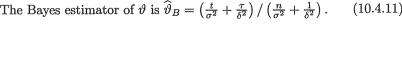
An arbitrary point estimator of  may be denoted by δ ≡ δ(T) which takes the value δ(t) when one observes T = t, t T. Suppose that the loss in estimating
  by the estimator θ(T) is given by
which is referred to as the squared error loss.
The mean squared error (MSE) discussed in Section 7.3.1 will correspond to the weighted average of the loss function from (10.4.1) with respect to the weights assigned by the pmf or pdf g(t; θ). In other words, this average is actually a conditional average given that  = θ. Let us define, conditionally given that
  = θ, the risk function associated with the estimator θ:
This is the frequentist risk which was referred to as MSEd in the Section 7.3. In Chapter 7, we saw examples of estimators δ1 and δ2 with risk functions R*(θ, δi), i = 1, 2 where R*(θ, δ1) > R*(θ, δ2) for some parameter values θ whereas R*(θ, δ1) ≤ R*(θ, δ2) for other parameter values θ. In other words, by comparing the two frequentist risk functions of δ1 and δ2, in some situations one may not be able to judge which estimator is decisively superior.
The prior h(θ) sets a sense of preference and priority of some values of v over other values of  . In a situation like this, while comparing two estimators δ1 and δ2, one may consider averaging the associated frequentist
486 10. Bayesian Methods
risks R*(θ, δi), i = 1, 2, with respect to the prior h(θ) and then check to see which weighted average is smaller. The estimator with the smaller average risk should be the preferred estimator.
So, let us define the Bayesian risk (as opposed to the frequentist risk)
Suppose that D is the class of all estimators of  whose Bayesian risks are finite. Now, the best estimator under the Bayesian paradigm will be δ* from D such that
Such an estimator will be called the Bayes estimator of  . In many standard problems, the Bayes estimator δ* happens to be unique.
Let us suppose that we are going to consider only those estimators δ and prior h(θ) so that both R*(θ, δ) and r*(v, δ) are finite, θ Θ.
Theorem 10.4.1 The Bayes estimator δ* = δ*(T) is to be determined in such a way that the posterior risk of δ*(t) is the least possible, that is
for all possible observed data t T.
Proof Assuming that m(t) > 0, let us express the Bayesian risk in the following form:
In the last step, we used the relation g(t; θ)h(θ) = k(t; θ)m(t) and the fact that the order of the double integral ∫Θ ∫T can be changed to ∫T ∫Θ because the integrands are non-negative. The interchanging of the order of the integrals is allowed here in view of a result known as Fubini’s Theorem which is stated as Exercise 10.4.10 for the reference.
Now, suppose that we have observed the data T = t. Then, the Bayes estimate δ*(t) must be the one associated with the
that is the smallest posterior risk. The proof is complete. !
An attractive feature of the Bayes estimator δ* is this: Having observed T = t, we can explicitly determine δ*(t) by implementing the process of minimizing the posterior risk as stated in (10.4.5). In the case of the squared
 In (10.4.8) we used the fact that
  as a function of
  =
=  is the unknown probability of success, 0 <
  < 1. Given that
  =
=  is minimal sufficient for
  is Beta(
 would be the mean of the posterior distribution, namely, the mean of the Beta(
 =
= 
488 10. Bayesian Methods
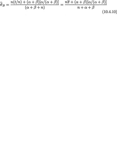
distribution is α/(α + β). The Bayes estimator is an appropriate weighted average of  and α/(α + β). If the sample size n is large, then the classical estimator
  gets more weight than the mean of the prior belief, namely α/(α + β) so that the observed data is valued more. For small sample sizes, gets less weight and thus the prior information is valued more. That is, for large sample sizes, the sample evidence is weighed in more, whereas if the sample size is small, the prior mean of
  is trusted more. !
Example 10.4.2 (Example 10.3.5 Continued) Let X1, ..., Xn be iid N(θ, σ2) given that v = θ, where  ( ) is the unknown population mean and σ(> 0) is assumed known. Consider the statistic
  which is minimal sufficient for θ given that
  = θ. Let us suppose that the prior distribution of v is N(τ, δ2) where τ( ) and β(> 0) are known numbers. From the Example 10.3.5, recall that the posterior distribution of
  is
is  where
where
 In view of the Theorem
10.4.2, under the squared error loss function, the Bayes estimator of  would be the mean of the posterior distribution, namely, the
  distribution. In other words, we can write:
Now, we can rewrite the Bayes estimator as follows:
From the likelihood function, that is given  = θ, the maximum likelihood estimate or the UMVUE of θ would be
  whereas the mean of the prior distribution is τ. The Bayes estimate is an appropriate weighted average of
  and τ. If n/σ2 is larger than 1/δ2, that is if the classical estimate
  is more reliable (smaller variance) than the prior mean τ, then the sample mean
  gets more weight than the prior belief. When n/σ2 is smaller than 1/δ2, the prior mean of v is trusted more than the sample mean
  . !
. !
10.5 Credible Intervals
Let us go back to the basic notions of Section 10.2. After combining the information about  gathered separately from two sources, namely the observed data X = x and the prior distribution h(θ), suppose that we have obtained the posterior pmf or pdf k(θ; t) of
  given T = t. Here, the statistic T is assumed to be (minimal) sufficient for θ, given that
  = θ.
= θ.
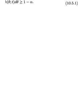
Definition 10.5.1 With fixed α, 0 < α < 1, a subset Θ* of the parameter space Θ is called a 100(1 – α)% credible set for the unknown parameter 
10. Bayesian Methods |
489 |
if and only if the posterior probability of the subset Θ* is at least (1 – α), that is
In some situations, a 100(1 – α)% credible set Θ*( Θ) for the unknown parameter  may not be a subinterval of Θ. The geometric structure of Θ* will largely depend upon the nature of the prior pdf h(θ) on Θ. When Θ* is an interval, we naturally refer to it as a 100(1 – α)% credible interval for
  .
.
10.5.1 Highest Posterior Density
It is conceivable that one will have to choose a 100(1 – α)% credible set Θ* from a long list of competing credible sets for v. Naturally, we should include only those values of v in a credible set which are “very likely” according to the posterior distribution. Also, the credible set should be “small” because we do not like to remain too uncertain about the value of v. The concept of the highest posterior density (HPD) credible set combines these two ideas.
Definition 10.5.2 With some fixed α, 0 < α < 1, a subset Θ* of the parameter space Θ is called a 100(1 – α)% highest posterior density (HPD) credible set for the unknown parameter v if and only if the subset Θ* has the following form:
where a ≡ a(α, t) is the largest constant such that the posterior probability of Θ is at least (1 – α).
Now, suppose that the posterior density k(θ; t) is unimodal. In this case, a 100(1 – α)% HPD credible set happens to be an interval. If we assume that the posterior pdf is symmetric about its finite mean (which would coincide with the its median too), then the HPD 100(1 – α)% credible interval Θ* will be the shortest as well as equal tailed and symmetric about the posterior mean. In order to verify this conclusion, one may apply the Theorem 9.2.1 in the context of the posterior pdf k(θ; t).
Example 10.5.1 (Examples 10.3.5 and 10.4.2 Continued) Let X1, ..., Xn be iid N(θ, σ2) given that  = θ where
  ( ) is the unknown population mean and s(> 0) is assumed known. Consider the statistic
  which is minimal sufficient for θ given that
  = θ. Let us suppose that the prior distribution of v is N(τ, δ2) where τ( ) and δ(>
0) are known numbers. From the Example 10.3.5, recall that the posterior distribution
490 10. Bayesian Methods
of  is
is  where
where 
Also, from the Example 10.4.2, recall that under the squared error loss function, the Bayes estimate of v would be the mean of the posterior distribution,
namely 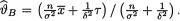 Let zα/2 stands for the upper 100(α/
2)% point of the standard normal distribution. The posterior distribution N(µ, σ20) being symmetric about µ, the HPD 100(1 – α)% credible interval Θ* will become
This interval is centered at the posterior mean  and it stretches either way by za/2 times the posterior standard deviation σ0. !
Example 10.5.2 (Example 10.5.1 Continued) In an elementary statistics course with large enrollment, the instructor postulated that the midterm examination score (X) should be distributed normally with an unknown mean θ
and variance 30, given that |
= θ. The instructor assumed the prior distribu- |
||||||||
tion N(73, 20) for |
and then looked at the midterm examination scores of n |
||||||||
= 20 randomly selected students. The observed data follows: |
|||||||||
85 |
78 |
87 |
92 |
66 |
59 |
88 |
61 |
59 |
78 |
82 |
72 |
75 |
79 |
63 |
67 |
69 |
77 |
73 |
81 |
One then has |
|
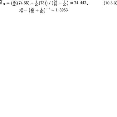
We wish to construct a 95% HPD credible interval |
|||||||
for the population average score v so that we have zα/2 = 1.96. The posterior mean and variance are respectively
From (10.5.3), we claim that the 95% HPD credible interval for  would be
which will be approximately the interval (72.127, 76.757). !
Example 10.5.3 (Example 10.4.1 Continued) Suppose that we have the random variables X1, ..., Xn which are iid Bernoulli(θ) given that v = θ where v is the unknown probability of success, 0< <1. Given that v = θ, the statistic
  is minimal sufficient for θ. Suppose that the prior distribution of
  is Beta(α, β) where α(>0) and β(> 0) are known numbers. From (10.3.2), recall that the posterior distribution of v is Beta(t + α, n – t + β) for t T = {0, 1, ..., n}. Using the Definition 10.5.2,
10. Bayesian Methods |
491 |
one can immediately write down the HPD 100(1 – α)% credible interval Θ* for  : Let us denote
with the largest positive number a such that P{Θ* |T = t) ≥ 1 – α. !
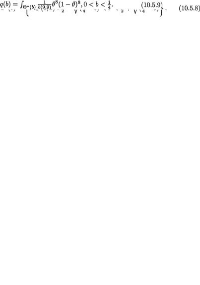
Example 10.5.4 (Example 10.5.3 Continued) In order to gather information about a new pain-killer, it was administered to n = 10 comparable patients suffering from the same type of headache. Each patient was checked after one-half hour to see if the pain was gone and we found seven patients reporting that their pain vanished. It is postulated that we have observed the random variables X1, ..., X10 which are iid Bernoulli(θ) given that  = θ where 0 <
  < 1 is the unknown probability of pain relief for each patient, 0 <
  < 1. Suppose that the prior distribution of
  was fixed in advance of data collection as Beta(2, 6). Now, we have observed seven patients who got the pain relief. From (10.5.5), one can immediately write down the form of the HPD 95% credible interval Θ* for
  as
as
with the largest positive number a such that P{Θ* |T = t) = 1 – α. Let us rewrite (10.5.6) as
We will choose the positive number b in (10.5.7) such that P{Θ*(b) |T = t) = 1 – α. We can simplify (10.5.7) and equivalently express, for 0 < b < ¼,
Now, the posterior probability content of the credible interval Θ*(b) is given by
We have given a plot of the function q(b) in the Figure 10.5.1. From this figure, we can guess that the posterior probability of the credible interval
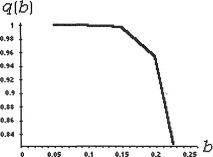
492 10. Bayesian Methods
Θ*(b) is going to be 95% when we choose b ≈ .2.
Figure 10.5.1. Plot of the Probability Content q(b) from (10.5.9)
With the help of MAPLE, we numerically solved the equation q(b) = .95 and found that b ≈ .20077. In other words, (10.5.8) will lead to the HPD 95% credible interval for v which is (.27812, .72188). !
10.5.2 Contrasting with the Confidence Intervals
Now, we emphasize important conceptual differences in the notions of a 100 (1–α)% confidence interval and a 100(1–α)% (HPD) credible interval for an unknown parameter  . In either case, one starts with an appropriate likelihood function. In the case of a confidence interval, the unknown parameter
  is assumed fixed. In the case of a credible interval, however, the unknown parameter
  is assumed to be a random variable having some pdf h(θ) on Θ. Under the frequentist paradigm, we talk about the unknown parameter
  belonging to a constructed confidence interval, only from the point of view of limiting relative frequency idea. Recall the interpretation given in Section 9.2.3. On the other hand, under the Bayesian paradigm we can evaluate the posterior probability that v belongs to a credible interval by integrating the posterior pdf on the interval. In this sense, the confidence coefficient may be regarded as a measure of initial accuracy which is fixed in advance by the experimenter whereas the posterior probability content of a credible interval may be regarded as the final accuracy. The latter conclusion may look more appealing in some applications but we may also remind the reader that a HPD credible interval arises at the expense of assuming that (i) the unknown parameter
 is a random variable and (ii)
  has a known prior distribution h(α) for α
Θ.
Example 10.5.5 (Example 10.5.2 Continued) With the sample of size n = 20 midterm examination scores, we had  and σ2 = 30. So
10. Bayesian Methods |
493 |
a 95% confidence interval for the population mean  would be 74.55 ±
 which will lead to the interval (72.15, 76.95). It is not meaningful for a frequentist to talk about the chance that the unknown parameter
  belongs or does not belong to the interval (72.15, 76.95) because
  is not a random variable. In order to make any such statement meaningful, the phrase “chance” would have to be tied in with some sense of randomness about v in the first place! A frequentist will add, however, that in a large collection of such confidence intervals constructed in the same fashion with n = 20, approximately 95% of the intervals will include the unknown value of
  .
.
On the other hand, the 95% HPD credible interval for  turned out to be (72.127, 76.757). Here, one should have no confusion about the interpretation of this particular interval’s “probability” content. The posterior pdf puts exactly 95% posterior probability on this interval. This statement is verifiable because the posterior is completely known once the observed value of the sample mean becomes available.
In this example, one may be tempted to say that the credible interval is more accurate than the confidence interval because it is shorter of the two. But, one should be very careful to pass any swift judgement. Before one compares the two intervals, one should ask: Are these two interval estimates comparable at all, and if they are, then in what sense are they comparable? This sounds like a very simple question, but it defies any simple answer. We may mention that philosophical differences between the frequentist and Bayesian schools of thought remains deep-rooted from the days of Fisher and Jeffreys. !
10.6 Tests of Hypotheses
We would like to recall that a concept of the p-value associated with the Neyman-Pearson’s frequentist theory of tests of hypotheses was briefly discussed in Section 8.4.1. In a Bayesian framework, one may argue that making a decision to reject or accept H0 based on the p-value is not very reasonable. Berger et al. (1997) gave an interesting exposition. A Bayes test of hypotheses is then formulated as follows.
Let us consider iid real valued random variables X1, ..., Xn having a common pmf or pdf f(x; v) where the unknown parameter  takes the values θ Θ ( ). We wish to test a null hypothesis H0 : v Θ0 against an alternative hypothesis H1 :
  Θ1 where Θ0 ∩ Θ1 = ϕ, Θ0 Θ1 Θ. Given
  = θ, we first write down the likelihood function
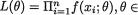
Θ and obtain the (minimal) sufficient statistic T ≡ T(X) which is assumed
494 10. Bayesian Methods
real valued. Let us continue to denote the prior of  and the pmf or pdf of T given
  = θ by h(θ) and g(t; θ) respectively.
Next, one obtains the posterior distribution k(θ; t) as in (10.2.3) and proceeds to evaluate the posterior probability of the null and alternative spaces Θ0, Θ1 respectively as follows:
We assume that both α0, α1 are positive and view these as the posterior evidences in favor of H0, H1 respectively.
We refrain from giving more details. One may refer to Ferguson (1967) and Berger (1985).
Example 10.6.1 (Example 10.3.5 Continued) Let X1, ..., X5 be iid N(θ, 4) given that  = θ where
  ( ) is the unknown population mean. Let us suppose that the prior distribution of v on the space Θ = is N(3, 1). We wish
to test a null hypothesis H0 : |
|
< 1 against an alternative hypothesis H1 : > |
||||
2.8. Consider the statistic |
|
|
which is minimal sufficient for θ given |
|||
that |
= θ. Suppose that the observed value of T is t = 6.5. |
|||||
With µ = ( --+ 3) (- + 1) |
-1 |
≈ 2. 0556 and |
the |
|||
|
6.5 |
5 |
|
|
|
|
|
4 |
4 |
|
|
|
|
posterior distribution of turns out to be |
Let us denote a random |
|||||
variable Y which is distributed as |
and Z = (Y – µ)/σ0. |
|||||
Now, from (10.6.1), we have α0 |
= P(Y < 1) = P(Z < -1. 5834) ≈ .0 5 6665 |
|||||
and α1 |
= P(Y > 2.8) = P(Z > 1. 1166) ≈ . 13208. Thus, the Bayes test from |
|||||
(10.6.2) will reject H0. ! |
|
|
|
|
||
So far, we have relied heavily upon conjugate priors. But, in some situations, a conjugate prior may not be available or may not seem very appealing. The set of examples in the next section will highlight a few such scenarios.
10.7 Examples with Non-Conjugate Priors
The following examples exploit some specific non-conjugate priors. Certainly these are not the only choices of such priors. Even though the chosen priors are non-conjugate, we are able to derive analytically the posterior and Bayes estimate.
Example 10.7.1 Let X be N(θ, 1) given that  =θ where
  is the unknown population mean. Consider the statistic T = X which is minimal
10. Bayesian Methods |
495 |
sufficient for θ given that  = θ. We have been told that
  is positive and so there is no point in assuming a normal prior for the parameter
  . For simplicity, let us suppose that the prior distribution of
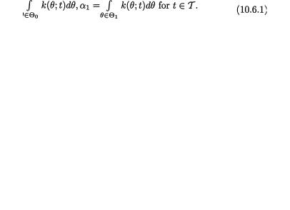
  on the space Θ = + is exponential with known mean α–1(> 0). Now, let us first proceed to determine the marginal pdf m(x). The joint distribution of (v, X) is given by
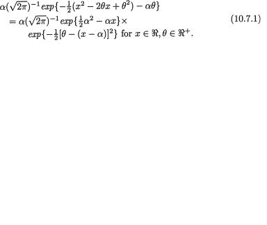
Recall the standard normal pdf  and the df
 with y . Thus, for all x , the marginal pdf of X can be written as
Now, combining (10.7.1)-(10.7.2), we obtain the posterior pdf of v given that X = x as follows: For all x , θ +,
In this example, the chosen prior is not a conjugate one and yet we have been able to derive the expression of the posterior pdf in a closed form. In the Exercise 10.7.1 we ask the reader to check by integration that k(θ; x) is indeed a pdf on the positive half of the real line. Also refer to the Exercises 10.7.2-10.7.3. !
Example 10.7.2 (Example 10.7.1 Continued) Let X be N(θ, 1) given that  = θ where v is the unknown population mean. Consider the statistic T = X which is minimal sufficient for θ given that
  = θ. We were told that
  was positive and we took the exponential distribution with the known mean α–1(> 0) as our prior for
  .
.
Let us recall the standard normal pdf  and the df
  for y . Now, from the Example 10.7.1, we know that the posterior distribution of v is given by k(θ; x) = {Φ ([x – α])}–1 φ(θ – [x – α]) for θ > 0, –∞ < x < ∞.
496 10. Bayesian Methods
In view of the Theorem 10.4.2, under the squared error loss function, the Bayes estimate of  would be the mean of the posterior distribution. In other words, one can write the Bayes estimate
  of
of  as
as
It is easy to check that I2 = x – α. Next, we rewrite I1 as
Now, combining (10.7.4)-(10.7.5), we get
as the Bayes estimate of  . Also refer to the Exercises 10.7.2-10.7.3. ! Example 10.7.3 (Example 10.7.2 Continued) Let X be N(θ, 1) given that
  = θ where
  is the unknown population mean. Consider the statistic T = X
which is minimal sufficient for θ given that  = θ. We were told that v was positive and we supposed that the prior distribution of
  was exponential with the known mean α–1(> 0). Under the squared error loss function, the Bayes estimate of
  turned out to be
  given by (10.7.6). Observe that the posterior distribution’s support is + and thus
  the mean of this posterior distribution, must be positive. But, notice that the observed data x may be larger or smaller than α. Can we check that the expression of
  will always lead to a positive estimate? The answer will be in the affirmative if we verify the following claim:
Note that  Φ(x) = φ(x) and
  φ(x) = –xφ(x) for all x . Thus, one has
 p(x) = Φ(x) which is positive for all x so that the function p(x) ↑ in x. Next, let us consider the behavior of p(x) when x is near negative infinity. By appealing to L’Hôpital’s rule from (1.6.29), we observe that
 Hence,
  Combine
10. Bayesian Methods |
497 |
this with the fact that p(x) is increasing in x( ) to validate (10.7.7). In other words, the expression of  is always positive. Also refer to the Exercises 10.7.2-10.7.3. !
In the three previous examples, we had worked with the normal likelihood function given  = θ. But, we were told that v was positive and hence we were forced to put a prior only on (0, ∞). We experimented with the exponential prior for
  which happened to be skewed to the right. In the case of a normal likelihood, some situations may instead call for a non-conjugate but symmetric prior for
  . Look at the next example.
Example 10.7.4 Let X be N(θ, 1) given that  = θ where
  ( ) is the unknown population mean. Consider the statistic T = X which is minimal sufficient for θ given that
  = θ. We have been told that (i)
  is an arbitrary real number, (ii)
  is likely to be distributed symmetrically around zero, and (iii) the prior probability around zero is little more than what it is likely with a normal prior. With the N(0, 1) prior on
  , we note that the prior probability of the interval (–.01, .01) amounts to 7.9787 × 10⁻³ whereas with the Laplace prior pdf h(θ) = ½e–|θ|I(θ ), the prior probability of the same interval amounts to 9.9502 × 10⁻³. So, let us start with the Laplace prior h(θ) for
  . From the apriori description of
  alone, it does not follow however that the chosen prior distribution is the only viable candidate. But, let us begin some preliminary investigation anyway.
One can verify that the marginal pdf m(x) of X can be written as
Next, one may verify that the posterior pdf of  given that X = x can be expressed as follows: For all x and θ ,
where b(x = {1 – Φ(x + 1)}exp{(x + 1)2/2}+F(x – 1)exp{(x – 1)2/2}. The details are left out as the Exercise 10.7.4. Also refer to the Exercises 10.7.5- 10.7.6. !
10.8Exercises and Complements
10.2.1Suppose that X1, ..., Xn are iid with the common pdf f(x; θ) = θe–θxI(x > 0) given that v = θ where v(> 0) is the unknown parameter.
498 10. Bayesian Methods
Assume the prior density h(θ) = ae–αθI(θ > 0) where α (> 0) is known. Derive the posterior pdf of v given that T = t where 
10.2.2 (Example 10.2.1 Continued) Suppose that X1, ..., X5 are iid with the common pdf f(x; θ) = θe-θxI(x > 0) given that  = θ where
  (> 0) is the unknown parameter. Assume the prior density h(θ) = 1/8e–θ/8I(θ > 0). Draw and compare the posterior pdf’s of
  given that
  with t = 15, 40, 50.
10.2.3 Suppose that X1, ..., Xn are iid Poisson(θ) given that  = θ where v(> 0) is the unknown population mean. Assume the prior density h(θ) = e– θI(θ > 0). Derive the posterior pdf of
  given that T = t where T =
10.2.4 (Example 10.2.3 Continued) Suppose that X1, ..., X10 are iid Poisson(θ) given that  = θ where
  (> 0) is the unknown population mean. Assume the prior density h(θ) = ¼e-θ/4I(θ > 0). Draw and compare the posterior pdf’s of
  given that with t = 30, 40, 50.
10.3.1Let X1, X2 be independent, X1 be distributed as N(θ, 1) and X2 be distributed as N(2θ, 3) given that  = θ where
  ( ) is the unknown parameter. Consider the minimal sufficient statistic T for θ given that
  = θ. Let us suppose that the prior distribution of
  on the space Θ = is N(5, τ2) where τ(> 0) is a known number. Derive the posterior distribution of v given that T
=t, t . {Hint: Given  = θ, is the statistic T normally distributed?}
10.3.2Suppose that X1, ..., Xn are iid Exponential(θ) given that  = θ where the parameter v(> 0) is unknown. We say that
  has the inverted gamma prior, denoted by IGamma(α, β), whenever the prior pdf is given by
where α, β are known positive numbers. Denote the sufficient statistic T =  given that
  = θ.
= θ.
(i) Show that the prior distribution of  is IGamma(α, β) if and only if
 has the Gamma(α, β) distribution;
(ii) Show that the posterior distribution of v given T = t turns out to be IGamma(n + α, {t + β-1}-1).
10.3.3 Suppose that X1, ..., Xn are iid N(0, θ2) given that  = θ where the parameter v(> 0) is unknown. Assume that
  2 has the inverted gamma prior IGamma(α, β), where α, β are known positive numbers. Denote the sufficient statistic
  given that
  = θ. Show that the posterior distribution of
  given T = t is an appropriate inverted gamma distribution.
10. Bayesian Methods |
499 |
10.3.4 Suppose that X1, ..., Xn are iid Uniform(0, θ) given that  = θ where the parameter
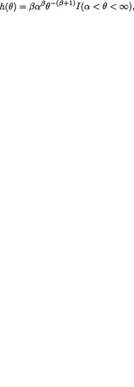
  (> 0) is unknown. We say that v has the Pareto prior, denoted by Pareto(α, β), when the prior pdf is given by
where α, β are known positive numbers. Denote the sufficient statistic T = Xn:n, the largest order statistic, given that  = θ. Show that the posterior distribution of v given T = t turns out to be Pareto(max(t, α), n + β).
10.3.5(Exercise 10.3.4 Continued) Let X1, ..., Xn be iid Uniform(0, aθ) given that  = θ where the parameter
  (> 0) is unknown, but a(> 0) is assumed known. Suppose that
  has the Pareto(α, β) prior where α, β are
known positive numbers. Denote the sufficient statistic T = Xn:n, the largest order statistic, given that  = θ. Show that the posterior distribution of
  given T = t is an appropriate Pareto distribution.
10.3.6Let X1, ..., Xn be iid Uniform(–θ, θ) given that  = θ where the parameter
  (> 0) is unknown. Suppose that
  has the Pareto(α, β) prior where α, β are known positive numbers. Denote the minimal sufficient statis-
tic T = |X|n:n, the largest order statistic among |X1|, ..., |Xn|, given that  = θ. Show that the posterior distribution of
  given T = t is an appropriate Pareto
distribution. {Hint: Can this problem be reduced to the Exercise 10.3.4?}
10.3.7Let X1, X2, X3 be independent, X1 be distributed as N(θ, 1), X2 be distributed as N(2θ, 3), and X3 be distributed as N(θ, 3) given that  = θ where
  ( ) is the unknown parameter. Consider the minimal sufficient statistic T for θ given that
  = θ. Let us suppose that the prior distribution of
  on the space Θ = is N(2, τ2) where τ(> 0) is a known number. Derive the posterior distribution of
  given that T = t, t . {Hint: Given
  = θ, is the statistic T normally distributed?}
10.3.8We denote  and suppose that X1, ..., Xn are iid N(θ1, θ 22) given that
  = θ where the parameters
  1( ),
1( ),  2( +) are assumed both unknown. Consider the minimal sufficient statistic T =
for θ given that  = θ. We are given the joint prior distribution of
  as follows:
where h½(θ1) stands for the pdf of the  distribution and
  stands for the pdf of the IGamma(2, 1) distribution. The form of the inverted gamma pdf was given in the Exercise 10.3.3.
500 |
10. Bayesian Methods |
|
|
|
||
(i) |
Given that |
= θ, write down the joint pdf of |
by taking the |
|||
|
product of the two separate pdf’s because these are independent, |
|||||
|
and this will serve as the likelihood function; |
|
|
|||
(ii) |
Multiply the joint pdf from part (i) with the joint prior pdf |
|||||
|
Then, combine the terms involving |
|
and the terms in- |
|||
|
volving only |
From this, conclude that the joint posterior pdf k(θ; |
||||
|
t) of |
given that |
that is |
|
can be viewed |
|
|
as |
|
|
Here, |
stands for the pdf (in |
|
|
the |
variable θ1) of |
the |
distribution with |
||
|
|
|
|
and |
|
stands for |
|
the pdf (in the variable θ 2) of the IGamma(α , β ) with α = 2 + ½n, |
|||||
|
β-01 = |
|
2 |
0 |
0 |
0 |
|
|
|
|
|
|
|
(iii) From the joint posterior pdf of  given that
  integrate out θ1 and thus show that the marginal posterior pdf of is the same as that of the IGamma(α0, β0) distribution as in part (ii);
(iv) From the joint posterior pdf of  given that
  integrate out
  and thus show that the marginal posterior pdf of θ1 is the same as that of an appropriate Student’s t distribution.
10.4.1 (Example 10.3.2 Continued) Let X1, ..., Xn be iid Poisson(θ) given that  = θ where v(> 0) is the unknown population mean. We suppose that the prior distribution of
  on the space Θ = (0, ∞) is Gamma(α, β) where α(> 0) and β(> 0) are known numbers. Under the squared error loss function, derive the expression of the Bayes estimate
  for
for  . {Hint: Use the form of the posterior from (10.3.3) and then appeal to the Theorem 10.4.2.}
10.4.2 (Exercise 10.3.1 Continued) Let X1, X2 be independent, X1 be distributed as N(θ, 1) and X2 be distributed as N(2θ, 3) given that  = θ where
  ( ) is the unknown parameter. Let us suppose that the prior distribution of
  on the space Θ = is N(5, τ2) where τ(> 0) is a known number. Under the squared error loss function, derive the expression of the Bayes estimate
  for
for  . {Hint: Use the form of the posterior from Exercise 10.3.1 and then appeal to the Theorem 10.4.2.}
10.4.3 (Exercise 10.3.2 Continued) Let X1, ..., Xn be iid Exponential(θ) given that  = θ where the parameter
  (> 0) is unknown. Assume that
  has the inverted gamma prior IGamma(α, β) where α, β are known positive numbers. Under the squared error loss function, derive the expression of
10. Bayesian Methods |
501 |
the Bayes estimate  for v. {Hint: Use the form of the posterior from Exercise 10.3.2 and then appeal to the Theorem 10.4.2.}
10.4.4(Exercise 10.3.3 Continued) Let X1, ..., Xn be iid N (0, θ2) given that v = θ where the parameter  (> 0) is unknown. Assume that
  has the inverted gamma prior IGamma(α, β) where α, β are known positive numbers. Under the squared error loss function, derive the expression of the Bayes
estimate  for
for  . {Hint: Use the form of the posterior from Exercise 10.3.3 and then appeal to the Theorem 10.4.2.}
10.4.5 (Exercise 10.3.4 Continued) Let X1, ..., Xn be iid Uniform (0, θ)
given that  = θ where the parameter v(> 0) is unknown. Suppose that
  has the Pareto(α, β) prior pdf h(θ) = βαβ θ-(β+1) I(α < θ < ∞) where α, β are
known positive numbers. Under the squared error loss function, derive the expression of the Bayes estimate  for
for  . {Hint: Use the form of the posterior from Exercise 10.3.4 and then appeal to the Theorem 10.4.2.}
10.4.6 (Exercise 10.3.5 Continued) Let X1, ..., Xn be iid Uniform (0, aθ) given that  = θ where the parameter
  (> 0) is unknown, but a(> 0) is assumed known. Suppose that
  has the Pareto(α, β) prior where α, β are known positive numbers. Under the squared error loss function, derive the expression of the Bayes estimate
  for
for  . {Hint: Use the form of the posterior from Exercise 10.3.5 and then appeal to the Theorem 10.4.2.}
10.4.7 (Exercise 10.3.6 Continued) Let X1, ..., Xn be iid Uniform(–θ, θ) given that  = θ where the parameter
  (> 0) is unknown. Suppose that v has the Pareto(α, β) prior where α, β are known positive numbers. Under the squared error loss function, derive the expression of the Bayes estimate
  for
for  . {Hint: Use the form of the posterior from Exercise 10.3.6 and then appeal to the Theorem 10.4.2.}
10.4.8 A soda dispensing machine is set up so that it automatically fills the soda cans. The actual amount of fill must not vary too much from the target (12 fl. ounces) because the overfill will add extra cost to the manufacturer while the underfill will generate complaints from the customers hampering the image of the company. A random sample of the fills for 15 cans gave  =0.14. Assuming a N (12, θ2) distribution for the actual fills given that v = θ(> 0) and the IGamma(10, 10) prior for
  2, obtain the Bayes estimate of the true population variance under the squared error loss.
10.4.9 Ten automobiles of the same make and model were driven by the drivers with similar road habits and the gas mileage for each was recorded over a week. The summary results included  miles per gallon. Assume a N (θ, 4) distribution for the actual gas mileage given that
  = θ ( ) and the N (20, 6) prior for
  . Construct a 90% HPD credible interval for the
502 10. Bayesian Methods
true average gas mileage per gallon,  . Give the Bayes estimate of the true average gas mileage per gallon
  under the squared error loss.
10.4.10 (Fubini’s Theorem) Suppose that a function of two real variables g(x1, x2) is either non-negative or integrable on the space χ = χ1 × χ2( ×). That is, for all (x1, x2) χ, the function g(x1, x2) is either non-negative or integrable. Then, show that the order of the (two-dimensional) integrals can be interchanged, that is, one can write
{Note: This is a hard result to verify. It is stated here for reference purposes and completeness. Fubini’s Theorem was used in the proof of the Theorem 10.4.1 for changing the order of two integrals.}
10.5.1 (Exercise 10.4.2 Continued) Let X1, X2 be independent, X1 be distributed as N (θ, 1) and X2 be distributed as N (2θ, 3) given that  = θ where
  ( ) is the unknown parameter. Let us suppose that the prior distribution of
  on the space Θ = is N (5, τ2) where τ(> 0) is a known number. With fixed 0 < α < 1, derive the 100(1 – α)% HPD credible interval for
  . {Hint: Use the form of the posterior from the Exercise 10.3.1.}
10.5.2 (Exercise 10.4.3 Continued) Let X1, ..., Xn be iid Exponential(θ) given that  = θ where the parameter
  (> 0) is unknown. Suppose that
  has the IGamma(1, 1) prior pdf h(θ) = θ–2 exp {–1/θ}I(θ > 0). With fixed 0 < α < 1, derive the 100(1 – α)% HPD credible interval for
  . {Hint: Use the form of the posterior from the Exercise 10.3.2.}
10.5.3 (Exercise 10.4.4 Continued) Let X1, ..., Xn be iid N (0, θ2) given that  = θ where the parameter v(> 0) is unknown. Suppose that
  has the IGamma(1, 1). With fixed 0 < α < 1, derive the 100(1 – α)% HPD credible interval for
  2. {Hint: Use the form of the posterior from the Exercise 10.3.3.}
10.5.4(Exercise 10.4.5 Continued) Let X1, ..., Xn be iid Uniform(0, θ) given that  = θ where the parameter
  (> 0) is unknown. Suppose that v has the Pareto(τ, β) prior, that is the prior pdf is given by h(θ) = βτβθ–(β+1) I(τ < θ
<∞) where τ, β are known positive numbers. With fixed 0 < α < 1, derive the 100(1 - a)% HPD credible interval for  . {Hint: Use the form of the posterior from the Exercise 10.3.4.}
10.5.5(Exercise 10.4.6 Continued) Let X1, ..., Xn be iid Uniform(0, aθ) given that  = θ where the parameter
  (> 0) is unknown, but a(> 0) is assumed known. Suppose that
  has the Pareto(τ, β) prior where τ, β are

10. Bayesian Methods |
503 |
known positive numbers. With fixed 0 < α < 1, derive the 100(1 – α)% HPD credible interval for  . {Hint: Use the form of the posterior from the Exercise 10.3.5.}
10.5.6 (Exercise 10.4.7 Continued) Let X1, ..., Xn be iid Uniform(–θ, θ) given that  = θ where the parameter
  (> 0) is unknown. Suppose that
  has the Pareto(τ, β) prior where τ, β are known positive numbers. With fixed 0 < α < 1, derive the 100(1 – α)% HPD credible interval for
  . Under the squared error loss function, derive the expression of the Bayes estimate
  for
for  . {Hint: Use the form of the posterior from the Exercise 10.3.6.}
10.5.7Suppose that X has its pdf f(x; θ) = 2θ–2 (θ – x)I(0 < x < θ) given that  = θ where the parameter
  (> 0) is unknown. Suppose that
  has the
Gamma(3, 2) distribution.
(i) Show that the posterior pdf k(θ x) = ¼ (θ – x)e–(θ–x)/2× I (0 < x < θ); (ii) With fixed 0 < α < 1, derive the 100(1 – α)% HPD credible interval
for  .
.
10.5.8(Exercise 10.3.7 Continued) Let X1, X2, X3 be independent, X1 be distributed as N (θ, 1), X2 be distributed as N (2θ, 3), and X3 be distributed as N (θ, 3) given that  = θ where
  ( ) is the unknown parameter. Consider the minimal sufficient statistic T for θ given that
  = θ. Let us suppose that the prior distribution of
  on the space Θ = is N (2, 9). Suppose that the following data has been observed:
Derive the 95% HPD credible interval for  . Under the squared error loss function, derive the expression of the Bayes estimate
  for
for  . {Hint: First find the posterior along the lines of the Exercise 10.3.7.}
10.6.1 (Example 10.6.1 Continued) Let X1, ..., X10 be iid N (θ, 4.5) given that  = θ where
  ( ) is the unknown parameter. Let us suppose that the prior distribution of
  on the space Θ = is N (4, 2). Consider the statistic
  which is minimal sufficient for θ given that
  = θ. Suppose that the observed value of T is t = 48.5. Use the Bayes test from (10.6.2) to choose between a null hypothesis H0 :
  < 3 against an alternative hypothesis
H1 :  ≥ 5.
≥ 5.
10.6.2 (Example 10.3.3 Continued) Let X1, X2, X3 be iid Bernoulli(θ) given that  = θ where
  is the unknown probability of success, 0 < v < 1. Let us assume that the prior distribution of v on the space Θ = (0, 1) is described as Beta(2, 4). Consider the statistic
  which is minimal sufficient for θ given that
  = θ. Suppose that the observed value of T is t = 2. Use the Bayes test from (10.6.2) to choose between a null hypothesis
504 10. Bayesian Methods
H0 :  ≤ .3 against an alternative hypothesis H1 :
  ≥ .5. {Hint: Use integration by parts when evaluating a0, a1 from (10.6.1). Review (1.6.28) as needed.} 10.6.3 (Example 10.3.4 Continued) Let X1, ..., X4 be iid Poisson(θ) given that v = θ where
  (> 0) is the unknown population mean. Let us suppose that the prior distribution of
  on the space Θ = (0, ∞) is Gamma(2, 3). Consider the statistic
  which is minimal sufficient for θ given that
  = θ. Suppose that the observed value of T is t = 1. Use the Bayes test from (10.6.2) to choose between a null hypothesis H0 :
  ≤ 1.5 against an alternative hypothesis H1 :
  ≥ 2.5. {Hint: Use integration by parts when evaluating α0, α1
from (10.6.1). Review (1.6.28) as needed.}
10.7.1(Example 10.7.1 Continued) Using the definition of a pdf, show that the function k(θ; x) given in (10.7.3) is indeed a probability density function of  .
.
10.7.2Let X1, ..., Xn be iid N (θ 1) given that  = θ where
  ( +) is the unknown parameter. Let us suppose that the prior pdf of
  on the space Θ =+ is given by h(θ) = αe–αθ I(θ > 0) where α(> 0) is a known number. Con-
sider  the sample mean, which is minimal sufficient for θ given that
Derive the marginal pdf m(t) of T for t ;
Derive the posterior pdf k(θ t) for v given that T = t, for θ > 0 and
–∞ < t < ∞;
(iii) Under the squared error loss function, derive the Bayes estimate  and show, as in the Example 10.7.3, that
  can take only positive values.
{Hint: Proceed along the lines of the Examples 10.7.1-10.7.2.}
10.7.3 (Exercise 10.7.2 Continued) Let X1, ..., X10 be iid N (θ, 1) given that  = θ where
  ( +) is the unknwon parameter. Let us suppose that the prior pdf of
  on the space Θ = + is given by h(θ) = αe-αθ I (θ > 0) where α(> 0) is a known number. Suppose that the observed value of the sample mean was 5.92. Plot the posterior pdf k(θ; t) assigning the values α = ½, ¼ and 1/8. Comment on the empirical behaviors of the corresponding posterior pdf and the Bayes estimates of
  .
.
10.7.4 (Example 10.7.4 Continued) Verify the expressions of m(x) and k(θ x) given by (10.7.8) and (10.7.9) respectively. Under the squared error loss function, derive the form of the Bayes estimate  .
.
10.7.5 Let X1, ..., Xn be iid N (θ, 1) given that  = θ where
  ( ) is the unknown parameter. Let us suppose that the prior pdf of
  on the space Θ =is given by h(θ) = ½αe-α|θ| I (θ ) where α(> 0) is a known number. Consider
  the sample mean, which is minimal sufficient for
10. Bayesian Methods |
505 |
θ given that  = θ.
= θ.
(i) Derive the marginal pdf m(t) of T for t ;
(ii) Derive the posterior pdf k(θ t) for v given that T = t, for θ > 0 and
–∞ < t < ∞;
(iii) Under the squared error loss function, derive the Bayes estimate  and show, as in the Example 10.7.3, that
  can take only positive values.
{Hint: Proceed along the Example 10.7.4.}
10.7.6 (Exercise 10.7.5 Continued) Let X1, ..., X10 be iid N (θ, 1) given that  = θ where
  ( ) is the unknown parameter. Let us suppose that the prior pdf of
  on the space Θ = is given by h(θ) = ½αe–α|θ| I (θ ) where α(> 0) is a known number. Suppose that the observed value of the sample mean was 5.92. Plot the posterior pdf k(θ t) assigning the values α = ½, ¼ and 1/8. Comment on the empirical behaviors of the corresponding posterior pdf and
the Bayes estimates of  .
.
This page intentionally left blank