

 which is interpreted as the best evidence in favor
508 11. Likehood Ratio and Other Tests
Note that small values of Λ are associated with the small values of 
relative to  If the best evidence in favor of the null hypothesis ap-
pears weak, then the null hypothesis is rejected. That is, we reject H0 for significantly small values of Λ.
It is easy to see that one must have 0 < Λ < 1 because in the definition of Λ, the supremum in the numerator (denominator) is taken over a smaller (larger) set Θ0(Θ). The cut-off number k (0, 1) has to be chosen in such a way that the LR test from (11.1.3) has the required level α.
For simplicity, we will handle only a special kind of null hypothesis. Let us test
where  is a known and fixed value of the (sub-) parameter θ1. One may be tempted to say that the hypothesis H0 is a simple null hypothesis. But, actually it may not be so. Even though H0 specifies a fixed value for a single component of θ, observe that the other components of ? remain unknown and arbitrary.
How should we evaluate |
First, in the expression of L(θ), we |
must plug in the value in the place of  . Then, we maximize the likelihood function L(
 , θ2, ..., θp) with respect to the (sub-) parameters θ2, ..., θp by substituting their respective MLE’s when we know that θ1 =
  On the other
hand, the |
is found by plugging in the MLE’s of all the components |
θ1, ..., θp in the likelihood function. In the following sections, we highlight these step by step derivations in a variety of situations.
Section 11.2 introduces LR tests for the mean and variance of a normal population. In Section 11.3, we discuss LR tests for comparing the means and variances of two independent normal populations. In Section 11.4, under the assumption of bivariate normality, test procedures are given for the population correlation coefficient ? and for comparing the means as well as variances.
11.2 One-Sample Problems
We focus on a single normal population and some LR tests associated with it. With fixed α (0,1), first a level α LR test is derived for a specified population mean against the two-sided alternative hypothesis, and come up with the customary two-sided Z-test (t-test) when the population variance is assumed known (unknown). Next, we obtain a level α LR test for
11. Likehood Ratio and Other Tests |
509 |
a specified population variance against the two-sided alternative hypothesis, and come up with the customary two-sided ?2-test assuming that the population mean is unknown.
11.2.1 LR Test for the Mean
Suppose that X1, ..., Xn are iid observations from the N(µ, σ2) population where µ , σ +. We assume that µ is unknown. Given α (0,1), consider choosing between a null hypothesis H0 : µ = µ0 and a two-sided alternative hypothesis H1 : µ ≠ µ0 with level α where µ0 is a fixed real number. We address the cases involving known σ or unknown σ separately. As usual,
 respectively denote the sample mean and variance.
Variance Known
Since σ is known, we have θ = µ, Θ0 = {µ0} and Θ = . In this case, H0 is a simple null hypothesis. The likelihood function is given by
Observe that
since Θ0 has the single element µ0. On the other hand, one has
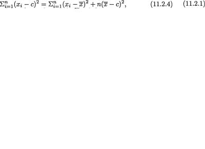
Note that for any real number c, we can write
and hence by combining (11.2.2)-(11.2.3) we obtain the likelihood ratio
Intuitively speaking, one may be inclined to reject H0 if and only if 
L(µ) is small or  is large. But for some data,
  and
and

510 11. Likehood Ratio and Other Tests
may be small or large at the same time. Thus, more formally, one rejects H0 if and only if Λ is small. Thus, we decide as follows:
where k(> 0) is a generic constant. That is, we reject H0 if and only if  is too large (>
  ) or too small (< –
  ). The implementable form of the level α LR test will look like this:
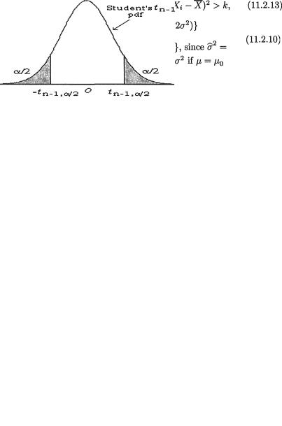
Figure 11.2.1. Two-Sided Standard Normal Rejection Region
See the Figure 11.2.1. The level of the two-sided Z-test (11.2.7) can be evaluated as follows:
which is α since  is distributed as N(0, 1) if µ = µ0.
From Section 8.5.1, recall that no UMP test exists for this problem.
Variance Unknown
We have θ = (µ, σ2), Θ0 = {(µ0, σ2) : µ0 is fixed, σ +} and Θ = {(µ, σ2) : µ , σ +}. In this case, H0 is not a simple null hypothesis. We assume
that the sample size n is at least two. The likelihood function is given by
 when properly scaled becomes too large or too small. The implementable form of the level
512 11. Likehood Ratio and Other Tests
See the Figure 11.2.2. The level of the two-sided t test (11.2.14) can be evaluated as follows:
which is α since  has the Student’s t distribution with n – 1 degrees of freedom if µ = µ0.
In principle, one may think of a LR test as long as one starts with the likelihood function. The observations do not need to be iid.
Look at the Exercises 11.2.6 and 11.2.9.
Example 11.2.1 In a recent meeting of the association for the commuting students at a college campus, an issue came up regarding the weekly average commuting distance (µ). A question was raised whether the weekly average commuting distance was 340 miles. Ten randomly selected commuters were asked about how much (X) each had driven to and from campus in the immediately preceding week. The data follows:
351.9 357.5 360.1 370.4 323.6 332.1 346.6 355.5 351.0 348.4
One obtains  miles and s = 13.4987 miles. Assume normality for the weekly driving distances. We may like to test H0 : µ = 340 against H1 : µ ≠ 340 at the 10% level. From (11.2.14), we have the observed value of the test statistic:
With α = .10 and 9 degrees of freedom, one has t9,.05 = 1.8331. Since |tcalc| exceeds t9,.05, we reject the null hypothesis at the 10% level. In other words, at the 10% level, we conclude that the average commuting distance per week is
significantly different from 340 miles. !
11.2.2 LR Test for the Variance
Suppose that X1, ..., Xn are iid observations from the N(µ, σ2) population where µ , σ +. We assume that both µ and σ are unknown. Given α (0, 1), we wish to find a level α LR test for choosing between a null hypothesis H0 : σ = σ0 and a two-sided alternative hypothesis H1 : σ ≠ σ0 where σ0 is a fixed positive real number. In this case, H0 is not a simple null hypothesis. As usual, we denote the sample mean 
and the sample variance  We have

11. Likehood Ratio and Other Tests |
513 |
θ = (µ, σ2), Θ0 = {(µ,  ) : µ , σ0 is fixed} and Θ = {(µ, σ2) : µ , σ+}.
The likelihood function is again given by
Now, observe that
On the other hand, one has 
from (11.2.11) where  Now, we combine this with (11.2.17) to obtain the likelihood ratio
Now, one rejects H0 if and only if ? is small. Thus, we decide as follows:
where k(> 0) is a generic constant.
Figure 11.2.3. Plot of the g(u) Function
In order to express the LR test in an implementable form, we proceed as follows: Consider the function g(u) = ue1-u for u > 0 and investigate
514 11. Likehood Ratio and Other Tests
its behavior to check when it is small (< k). We note that g(1) = 1 and g (u) = {(1 - u)/u}g(u) which is positive (negative) when u < 1 (u > 1). Hence, the function g(u) is strictly increasing (decreasing) on the left (right) hand side of u = 1. Thus, g(u) is going to be “small” for both very small and very large values of u(> 0). This feature is also clear from the plot of the function g(u) given in the Figure 11.2.1. Thus, we rewrite the LR test (11.2.19) as follows:
as long a, b as are chosen so that the test has level α.
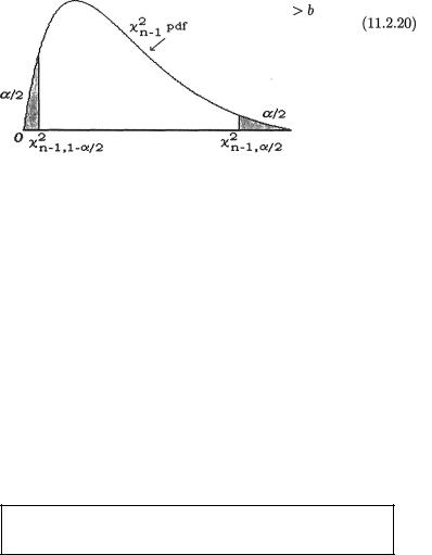
Figure 11.2.4. Two-Sided  Rejection Region
Recall that  has a Chisquare
distribution with n – 1 degrees of freedom if σ = σ0 and hence a level α LR test can be expressed as follows:
That is, we reject H0 if and only if  when properly scaled becomes too large or too small. See the Figure 11.2.4. The case when µ is known has been left as the Exercises 11.2.2-11.2.3. Also look at the related Exercise 11.2.4.
Recall from the Exercise 8.5.5 that no UMP level α test exists for testing H0 versus H1 even if µ is known.
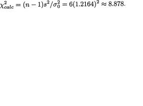
Example 11.2.2 In a dart-game, the goal is to throw a dart and hit the bull’s eye at the center. After the dart lands on the board, its distance (X)
 inches and
  and
and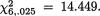 Since
Since  lies between the two numbers 1.2373 and 14.449, we accept
  and
and  lies outside of the interval (10.117, 30.144), one should
516 11. Likehood Ratio and Other Tests
parameters are unknown and θ = (µ1, µ2, σ) × × +. Given α (0, 1), we wish to find a level α LR test for choosing between a null hypothesis H0 : µ1 = µ2 and a two-sided alternative hypothesis H1 : µ1 ≠ µ2. With ni ≥ 2, let us denote
for i = 1, 2. Here,  is the pooled estimator of σ2.
Since H0 specifies that the two means are same, we have Θ0 = {(µ, µ, σ2):
µ , σ +}, and Θ = {(µ1, µ2, σ2) : µ1 , µ2 , σ +}. The likelihood function is given by
Thus, we can write
One should check that the maximum likelihood estimates of µ, σ2 obtained from this restricted likelihood function turns out to be
Hence, from (11.3.3)-(11.3.4) we have
On the other hand, one has
 from (11.3.4) and reject
 will correspond to the “large” values of
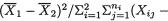
 Thus, we can rewrite the test (11.3.8) as follows:
518 11. Likehood Ratio and Other Tests
From Example 4.5.2 recall that  has the
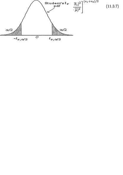
Student’s t distribution with n1 + n2 – 2 degrees of freedom. Thus, in view of (11.3.10), the implementable form of a level α LR test would be:
See the Figure 11.3.1. Note that the LR test rejects H0 when  is sizably different from zero with proper scaling.
Look at the Exercises 11.3.2-11.3.3 for a LR test of the equality of means in the case of known variances.
Look at the Exercises 11.3.4-11.3.6 for a LR test to choose between H0 : µ1 – µ2 = D versus H1 : µ1 – µ2 ≠ D.
Example 11.3.1 Weekly salaries (in dollars) of two typical high-school seniors, Lisa and Mike, earned during last summer are given below:
Lisa: 234.26, 237.18, 238.16, 259.53, 242.76, 237.81, 250.95, 277.83 Mike: 187.73, 206.08, 176.71, 213.69, 224.34, 235.24
Assume independent normal distributions with unknown average weekly salaries, µL for Lisa and µM for Mike, but with common unknown variance σ2. At 5% level we wish to test whether the average weekly salaries are same for these two students, that is we have to test H0 : µL = µM versus H1 : µL ≠ µM. One has
so that the pooled sample variance
From (11.3.11), we find the observed value of the test statistic:
With α = .05 and 12 degrees of freedom, we have t12,.025 = 2.1788. Since |tcalc| exceeds t12,.025, we reject the null hypothesis at 5% level. At 5% level, we conclude that the average weekly salaries of Lisa and Mike were signifi-
cantly different. !

 ),
),  , and for
  :
:  × ×
× × 
520 11. Likehood Ratio and Other Tests
On the other hand, one has
Now, we combine (11.3.16)-(11.3.17) to express the likelihood ratio as
where a ≡ a(n1, n2), b = b(n1, n2) are positive numbers which depend on n1, n2 only. Now, one rejects H0 if and only if is small. Thus, we decide as follows:
or equivalentl |
y, |
where k(> 0) is a generic constant.
In order to express the LR test in an implementable form, we proceed as follows: Consider the function g(u) = un1/2(u + b) –n1+n2)/2 for u > 0 and investigate its behavior in order to check when it is small (< k). Note that g′(u) = ½u(n–2)/2 (u +b)–(n1+n2+2)/2{n1b – n2u} which is positive (negative) when u <
(>)n1b/n2. Hence, g(u) is strictly increasing (decreasing) on the left (right) hand side of u = n1b/n2. Thus, g(u) is going to be “small” for both very small or very large values of u(> 0).
Next, we rewrite the LR test (11.3.19) as follows:
11. Likehood Ratio and Other Tests |
521 |
where the numbers c, d are chosen in such a way that the test has level α.
Figure 11.3.2. Two-Sided Fn1-1,n2-1 Rejection Region
Recall that  has the F distribution with the degrees of freedom n1 – 1, n2
– 1 when σ1 = σ2, that is under the null hypothesis H0. Hence, a level α LR test can be written as follows:
Thus, this test rejects H0 when  is sizably different from one. See the Figure 11.3.2.
Look at the Exercises 11.3.9-11.3.10 for a LR test of the equality of variances in the case of known means.
Look at the Exercise 11.3.11 for a LR test to choose between H0 : σ1/σ2 = D(> 0) versus H1 : σ1/σ2 ≠ D.
Example 11.3.2 Over a period of 6 consecutive days, the opening prices (dollars) of two well known stocks were observed and recorded as follows:
Stock #1: 39.09, 39.70, 41.77, 38.96, 41.42, 42.26 Stock #2: 42.33, 39.16, 42.10, 40.92, 46.47, 45.02
Let us make a naive assumption that the two stock prices went up or down independently during the period under study. The stock prices gave rise to
and the question we want to address is whether the variabilities in the opening prices of the two stocks are the same at 10% level. That is, we want to test H0 : σ1 = σ2 versus the two-sided alternative hypothesis

522 11. Likehood Ratio and Other Tests
H1 : σ1 ≠ σ2. Assume normality. From (11.3.21), we find the observed value of the test statistic:
With α = .10, one has F5,5,.05 = 5.0503 and F5,5,.95 =  .19801. Since Fcalc lies between the two numbers. 19801 and 5.0503, we conclude at 10% level
that the two stock prices were equally variable during the six days under investigation. !
The problem of testing the equality of means of two independent normal populations with unknown and unequal variances is hard. It is referred to as the Behrens-Fisher problem. For some ideas and references, look at both the Exercises 11.3.15 and 13.2.10.
11.4 Bivariate Normal Observations
We have discussed LR tests to check the equality of means of two independent normal populations. In some situations, however, the two normal populations may be dependent. Recall the Example 9.3.3. Different test procedures are used in practice in order to handle such problems.
Suppose that the pairs of random variables (X1i, X2i) are iid bivariate normal, N2(µ1, µ2,  ρ), i = 1, ..., n(≥ 2). Here we assume that all five parameters are unknown, (µl, σl) × +, l = 1, 2 and –1 < ρ < 1. Test procedures are summarized for the population correlation coefficient ρ and for comparing the means µ1, µ2 as well as the variances
  .
.
11.4.1 Comparing the Means: The Paired Difference t Method
With fixed α (0, 1), we wish to find a level α test for a null hypothesis H0 : µ1 = µ2 against the upper-, lower-, or two-sided alternative hypothesis H1. The methodology from the Section 11.3.1 will not apply here. Let us denote
Observe that Y1, ..., Yn are iid N(µ1 - µ2, σ2) where σ2 =  – 2ρσ1σ2. Since the mean µ1 – µ2 and the variance σ2 of the common normal distribu-
tion of the Y’s are unknown, the two-sample problem on hand is reduced

 = –4.625,
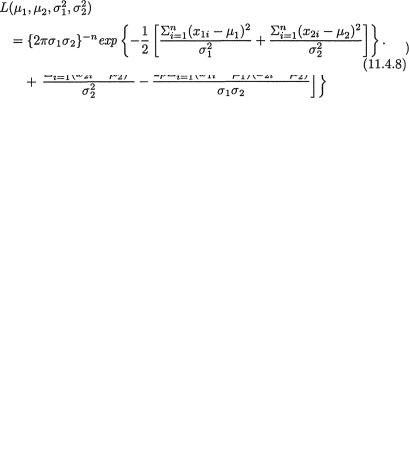
11. Likehood Ratio and Other Tests |
525 |
With α = .01 and 7 degrees of freedom, one has t7,.01 = 2.9980. But, since ucalc does not go below –t7,.01, we do not reject the null hypothesis at 1% level. In other words, at 1% level, we conclude that the job training has not been
effective. !
11.4.2 LR Test for the Correlation Coefficient
With fixed α (0, 1), we wish to construct a level α LR test for a null hypothesis H0 : ρ = 0 against a two-sided alternative hypothesis H1 : ρ ≠ 0. We
denote θ = (µ1, µ2,  ρ) and write Θ0 = {(µ1, µ2,
  0) : µ1 , µ2
, σ1 +, σ2 +}, and Θ = {(µ1, µ2,  ρ) : µ1 , µ2 , σ1 +, σ2 +, ρ (-1, 1)}. The likelihood function is given by
for all θ Θ. We leave it as Exercise 11.4.5 to show that the MLE’s for µ1, µ2,
 and ρ are respectively given by
 and
and 
These stand for the customary sample means, sample variances (not unbiased), and the sample correlation coefficient. Hence, from (11.4.6) one has
Under the null hypothesis, that is when ? = 0, the likelihood function happens to be
We leave it as the Exercise 11.4.4 to show that the MLE’s for µ1, µ2,  and
and  are respectively given by
 These again stand for the customary sample means and sample variances (not unbiased). Hence, from (11.4.8) one has
526 11. Likehood Ratio and Other Tests
Now, one rejects H0 if and only if Λ is small. Thus, we decide as follows:
or equivalently
where k(> 0) is a generic constant. Note that r2/(1 - r2) is a one-to-one function of r2. It is easy to see that this test rejects H0 when r is sizably different from zero.
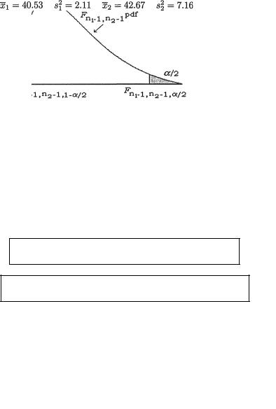
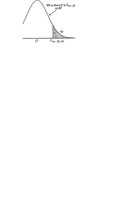
Figure 11.4.4. Two-Sided Student’s tn-2 Rejection Region
Now, recall from (4.6.10) that  has the Student’s t distribution with n – 2 degrees of freedom when ρ = 0. This is why we assumed that n was at least three. The derivation of this sampling distribution was one of the earliest fundamental contributions of Fisher (1915). See the Figure 11.4.4. Now, from (11.4.10), a level α LR test can be expressed as follows:
Upper-Sided Alternative Hypothesis
We test H0 : ρ = 0 versus H1 : ρ > 0. See the Figure 11.4.5. Along the lines of (11.4.11), we can propose the following upper-sided level α test:
11. Likehood Ratio and Other Tests |
527 |
Figure 11.4.5. Upper-Sided Student’s tn-2 Rejection Region
Lower-Sided Alternative Hypothesis
We test H0 : θ = 0 versus H1 : ρ < 0. See the Figure 11.4.6. Along the lines of (11.4.11), one can also propose the following lower-sided level α test:
Figure 11.4.6. Lower-Sided Student’s tn-2 Rejection Region
Example 11.4.2 (Example 11.4.1 Continued) Consider the data on (X1, X2) from Example 11.4.1 for 8 employees on their job performance scores before and after the training. Assuming a bivariate normal distribution for (X1, X2), we wish to test whether the job performance scores before and after the training are correlated. At 10% level, first we may want to test H0 : ρ = 0 versus H1 : ρ ≠ 0. For the observed data, one should check that r = .837257. From (11.4.11), we find the observed value of the test statistic:
528 11. Likehood Ratio and Other Tests
With α = .10 and 6 degrees of freedom, one has t6,.05 = 1.9432. Since |tcalc| exceeds t6,.05, we reject the null hypothesis at 10% level and conclude that the job performance scores before and after training appear to be significantly
correlated. !
11.4.3 Test for the Variances
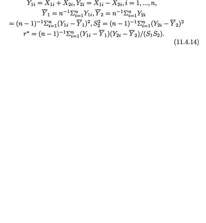
With fixed α (0, 1), we wish to construct a level α test for the null hypothesis H0 : σ1 = σ2 against the upper-, lower-, or two-sided alternative hypothesis H1. The methodology from Section 11.3.2 does not apply. Let us denote
Observe that (Y1i, Y2i) are iid bivariate normal, N2(ν1, ν2,  ρ*), i = 1, ..., n(≥ 3) where ν1 = µ1 + µ2, ν2 = µ1 – µ2,
 and Cov(Y1i, Y2i) =
  so that ρ* = (
 )/(τ1τ2). Of course all the parameters ν1, ν2,
  ρ* are unknown, (νl, τl) × +, l =
1, 2 and –1 < ρ* < 1.
Now, it is clear that testing the original null hypothesis H0 : σ1 = σ2 is equivalent to testing a null hypothesis H0 : ρ* = 0 whereas the upper-, lower- , or two-sided alternative hypothesis regarding σ1, σ2 will translate into an upper-, lower-, or two-sided alternative hypothesis regarding ρ*. So, a level α test procedure can be derived by mimicking the proposed methodologies from (11.4.11)-(11.4.13) once r is replaced by the new sample correlation coefficient τ* obtained from the transformed data (Y1i, Y2i), i = 1, ..., n(≥ 3).
Upper-Sided Alternative Hypothesis
We test H0 : σ1 = σ2 versus H1 : σ1 > σ2. See the Figure11.4.5. Along the lines of (11.4.12), we can propose the following upper-sided level α test:
Lower-Sided Alternative Hypothesis
We test H0 : σ1 = σ2 versus H1 : σ1 < σ2. See the Figure 11.4.6. Along


53011. Likehood Ratio and Other Tests
11.2.2Suppose that X1, ..., Xn are iid N(0, σ2) where σ(> 0) is the unknown parameter. With preassigned α (0, 1), derive a level α LR test for the
null hypothesis H0 : σ2 =  against an alternative hypothesis H1 :
  in the implementable form. {Note: Recall from the Exercise 8.5.5 that no UMP level α test exists for testing H0 versus H1}.
11.2.3 Suppose that X1, ..., Xn are iid N(µ, σ2) where σ ( +) is the unknown parameter but µ( ) is assumed known. With preassigned α (0, 1), derive a level α LR test for a null hypothesis H0 :  against an alternative hypothesis H1 :
  in the implementable form. {Note: Recall from the Exercise 8.5.5 that no UMP level a test exists for testing H0 versus
H1}.
11.2.4 Suppose that X1, X2 are iid N(µ, σ2) where µ( ), σ( +) are both assumed unknown parameters. With preassigned α (0, 1), reconsider the level α LR test from (11.2.21) for choosing between a null hypothesis H0 :  against an alternative hypothesis H1 :
  Show that the same test can be expressed as follows: Reject H0 if and only if |X1 – X2| >
11.2.5Suppose that X1, ..., Xn are iid having the common exponential pdf f(x; θ) = θ–1 exp{–x/θ}I(x > 0) where θ(> 0) is assumed unknown. With
preassigned α (0, 1), derive a level α LR test for a null hypothesis H0 : θ = θ0(> 0) against an alternative hypothesis H1 : θ ≠ θ0 in the implementable form. {Note: Recall from the Exercise 8.5.4 that no UMP level a test exists for testing H0 versus H1}.
11.2.6Suppose that X1 and X2 are independent random variables respectively distributed as N(µ, σ2), N(3µ, 2σ2) where µ is the unknown parameter and σ + is assumed known. With preassigned α (0, 1), derive a level
αLR test for H0 : µ = µ0 versus H1 : µ ≠ µ0 where µ0 ( ) is a fixed number, in the implementable form. {Hint: Write down the likelihood function along the line of (8.3.31) and then proceed directly as in Section 11.2.1.}
11.2.7Suppose that X1, ..., Xn are iid having the Rayleigh distribution with the common pdf f(x; θ) = 2θ–1 xexp(–x2/θ)I(x > 0) where θ(> 0) is the un-
known parameter. With preassigned α (0, 1), derive a level α LR test for H0 : θ = θ0 versus H1 : θ ≠ θ0 where θ0( +) is a fixed number, in the implementable form.
11.2.8Suppose that X1, ..., Xn are iid having the Weibull distribution with the common pdf f(x; a) = a–1bxb–1 exp(–xb/a)I(x > 0) where a(> 0) is an unknown parameter but b(> 0) is assumed known. With preassigned a (0,
1), derive a level α LR test for H0 : a = a0 versus H1 : a ≠ a0 where a0 is a positive number, in the implementable form.
11. Likehood Ratio and Other Tests |
531 |
11.2.9 Let us denote X′ = (X1, X2) where X is assumed to have the bivariate normal distribution, N2(µ, µ, 1, 2,  ). Here, we consider µ( ) as the
unknown parameter. With preassigned α (0, 1), derive a level α LR test for H0 : µ = µ0 versus H1 : µ ≠ µ0 where µ0 is a real number, in the implementable form. {Hint: Write down the likelihood function along the line of (8.3.33) and proceed accordingly.}
11.2.10Let X1, ..., Xn be iid positive random variables having the common lognormal pdf f(x; µ) =  exp {-[log(x) - µ]2/(2s2)} with x > 0, –∞ <
µ< ∞ 0 < σ < ∞. Here, µ is the only unknown parameter. With preassigned α
(0, 1), derive a level α LR test for H0 : µ = µ0 versus H1 : µ ≠ µ0 where µ0 is a real number, in the implementable form.
11.2.11Suppose that X1, ..., Xn are iid having the common Laplace pdf f(x; b) = ½b–1 exp( – |x – a| /b)I(x ) where b(> 0) is an unknown parameter but α( ) is assumed known. With preassigned α (0, 1), derive a level α LR
test for a null hypothesis H0 : b = b0(> 0) against the alternative hypothesis H1 : b ≠ b0 in the implementable form. {Hint: Use the Exercise 11.2.4.}
11.2.12Suppose that X1, ..., Xn are iid having the common negative exponential pdf f(x; µ) = σ–1 exp{–(x – µ)/σ}I(x > µ) where µ( ) is an unknown parameter but σ( +) is assumed known. With preassigned α (0, 1),
derive a level α LR test for H0 : µ = µ0 versus H1 : µ ≠ µ0 where µ0 is a real number, in the implementable form.
11.2.13Suppose that X1, ..., Xn are iid random variables having the common pdf f(x; θ) = θ–1x(1-θ)/1I(0 < x < 1) with 0 < θ < ∞. Here, θ is the unknown
parameter. With preassigned α (0, 1), derive a level α LR test for H0 : θ = θ0 versus H1 : θ ≠ θ0 where θ0 is a positive number, in the implementable form.
11.2.14A soda dispensing machine automatically fills the soda cans. The actual amount of fill must not vary too much from the target (12 fl. ounces) because the overfill will add extra cost to the manufacturer while the underfill will generate complaints from the customers. A random sample of the fills for 15 cans gave a standard deviation of .008 ounces. Assuming a normal distribution for the fills, test at 5% level whether the true population standard deviation is different from .01 ounces.
11.2.15Ten automobiles of the same make and model were used by drivers with similar road habits and the gas mileage for each was recorded over a week. The summary results were  = 22 miles per gallon and s = 3.5 miles per gallon. Test at 10% level whether the true average gas mileage per gallon is any different from 20.
11.2.16The waiting time (in minutes) for a passenger at a bus stop
532 11. Likehood Ratio and Other Tests
is assumed to have an exponential distribution with mean θ (> 0). The waiting times for ten passengers were recorded as follows in one afternoon:
6.2 |
5.8 |
4.5 |
6.1 |
4.6 |
4.8 |
5.3 |
5.0 |
3.8 |
4.0 |
Test at 5% level whether the true average waiting time is any different from 5.3 minutes. {Hint: Use the test from Exercise 11.2.5.}
11.3.1 Verify the expressions of the MLE’s in (11.3.4).
11.3.2 Let the random variables Xi1, ..., Xini be iid N(µi,  ), i = 1, 2, and that the X1j’s be independent of the X2j’s. Here we assume that µ1, µ2 are
unknown and (µ1, µ2) × but (σ1, σ2) + × + are assumed known. With preassigned α (0, 1), derive a level α LR test for H0 : µ1 = µ2 versus H1
: µ1 ≠ µ2 in the implementable form. {Hint: The LR test rejects H0 if and only if
11.3.3 Let the random variables Xi1, ..., Xini be iid N(µi, σ2), i = 1, 2, and that the X1j’s be independent of the X2j’s. Here we assume that µ1, µ2 are
unknown and (µ1, µ2) × but σ + is assumed known. With preassigned α (0, 1), derive a level α LR test for H0 : µ1 = µ2 versus H1 : µ1 ≠ µ2 in the implementable form. {Hint: The LR test rejects H0 if and only if
11.3.4 Let the random variables Xi1, ..., Xini be iid N(µi, σ2), i = 1, 2, and that the X1j’s be independent of the X2j’s. Here we assume that µ1, µ2, σ are all unknown and
(µ1, µ2) × , σ +. With preassigned α (0, 1) and a real number D, show that a level α LR test for H0 : µ1 – µ2 = D versus H1 : µ1 – µ2 ≠ D would reject H0 if and only if 
 {Hint: Re-
peat the techniques from Section 11.3.1.}
11.3.5 (Exercise 11.3.2 Continued) Let the random variables Xi1, ..., Xini be iid N(µi,  ), i = 1, 2, and that the X1j’s be independent of the X2j’s. Here we
assume that µ1, µ2 are unknown and (µ1, µ2) × but (σ1, σ2) + × + are assumed known. With preassigned α (0, 1) and a real number D, derive
a level α LR test for H0 : µ1 – µ2 = D versus H1 : µ1 – µ2 ≠ D in the implementable form. {Hint: The LR test rejects H0 if and only if
11.3.6 (Exercise 11.3.3 Continued) Let the random variables Xi1, ...,
Xini be iid N(µi, σ2), i = 1, 2, and that the X1j’s be independent of the X2j’s. Here we assume that µ1, µ2 are unknown and (µ1, µ2) × but σ +
is assumed known. With preassigned α (0, 1) and a real number D, derive a level α LR test for H0 : µ1 – µ2 = D versus H1 : µ1 – µ2 ≠ D
11. Likehood Ratio and Other Tests |
533 |
in the implementable form. {Hint: The LR test rejects H0 if and only if
11.3.7 Two types of cars were compared for the braking distances. Test runs were made for each car in a driving range. Once a car reached the stable speed of 60 miles per hour, the brakes were applied. The distance (feet) each car travelled from the moment the brakes were applied to the moment the car came to a complete stop was recorded. The summary statistics are shown below:
Car |
Sample Size |
|
s |
Make A |
nA = 12 |
37.1 |
3.1 |
Make B |
nB = 10 |
39.6 |
4.3 |
Assume that the elapsed times are distributed as N(µA, σ2) and N(µB, σ2) respectively for the make A and B cars with all parameters unknown. Test at 5% level whether the average braking distances of the two makes are significantly different.
11.3.8 Verify the expressions of the MLE’s in (11.3.15).
11.3.9 Let the random variables Xi1, ..., Xini be iid N(0,  ), i = 1, 2, and that the X1j’s be independent of the X2j’s. Here we assume that (µ1, µ2) × are
known but (σ1, σ2) + × + are unknown. With preassigned α (0, 1), derive a level α LR test for H0 : σ1 = σ2 versus H1 : σ1 ≠ σ2 in the implementable form.
11.3.10 Let the random variables Xi1, ..., Xini be iid N(µi,  ), i = 1, 2, and that the X1j’s be independent of the X2j’s. Here we assume that µ1, µ2) ×
are known but (σ1, σ2) + × + are unknown. With preassigned α (0, 1), derive a level α LR test for H0 : σ1 = σ2 versus H1 : σ1 ≠ σ2 in the implementable form.
11.3.11 Let the random variables Xi1, ..., Xini be iid N(µi,  ), i = 1, 2, and that the X1j’s be independent of the X2j’s. Here we assume that µ1, µ2, s1, s2 are
all unknown and (µ1, µ2) 2, (σ1, σ2) +2. With preassigned α (0, 1) and a positive number D, show that the level α LR test for H0 : σ1/σ2 = D
versus H1 : σ1/σ2 ≠ D, would reject H0 if and only if >  Fn1 - 1,n2 - 1,α/ 2 or <
  Fn1 - 1,n2 -1,1 - α/2. {Hint: Repeat the techniques from Section
11.3.2.}
11.3.12Let the random variables Xn1, ..., Xini be iid Exponential(θi), i = 1, 2, and that the X1j’s be independent of the X2j’s. Here we assume that θ1, θ2 are unknown and (θ1, θ2) + × +. With preassigned α (0, 1), derive a level α LR test for H0 : θ1 = θ2 versus H1 : θ1 ≠ θ2 in the
534 11. Likehood Ratio and Other Tests
implementable form. {Hint: Proceed along Section 11.3.2. With 0 < c < d < ∞, a LR test rejects H0 if and only if  < c or > d.}
11.3.13 Two neighboring towns wanted to compare the variations in the time (minutes) to finish a 5k-run among the first place winners during each town’s festivities such as the heritage day, peach festival, memorial day, and other town-wide events. The following data was collected recently by these two towns:
Town A (xA): |
18 |
20 |
17 |
22 |
19 |
18 |
20 18 17 |
Town B (xB): |
20 |
17 |
25 |
24 |
18 |
23 |
|
Assume that the performances of the first place winners are independent and that the first place winning times are normally distributed within each town. Then, test at 1% level whether the two town’s officials may assume σA = σB.
11.3.14 Let the random variables Xi1, ..., Xini be iid N(µi, ∞2), ni ≥ 2, i = 1, 2, 3 and that the X1j’s, X2j’s and X2j’s be all independent. Here we assume that
µ1, µ2, µ3, ∞ are all unknown and (µ1, µ2, µ3) 3, ∞ +. With preassigned α (0, 1), show that a level α LR test for H0 : µ1 + µ2 = 2µ3 versus H1 : µ1 + µ2 ≠ 2µ3 would reject H0 if and only if
 where
where  is understood to be the corresponding pooled sample variance based on n1 + n2 + n3 – 3 degrees of freedom. {Hint: Repeat the techniques from Section 11.3.1. Under H0, while writing down the likelihood function, keep µ1, µ2 but replace µ3 by ½(µ1 + µ2) and maximize the likelihood function with respect to µ1, µ2 only.}
11.3.15 (Behrens-Fisher problem) Let Xi1, ..., Xini be iid N(µi,  ) random variables, ni ≥ 2, i = 1, 2, and that the X1j’s be independent of the X2j’s. Here we
assume that µ1, µ2, σ1, σ2 are all unknown and (µ1, µ2) 2, (σ1, σ2) +2, σ1 ≠ σ2. Let  respectively be the sample mean and variance, i = 1, 2. With
preassigned α (0, 1), we wish to have a level a test for H0 : µ1 = µ2 versus H1 : µ1 ≠ µ2 in the implementable form. It may be natural to use the test statistic
Ucalc where  Under H0, the statistic Ucalc has approximately a Student’s
  distribution with
 Obtain a two-sided approximate t test based on
Ucalc. {Hint: This is referred to as the Behrens-Fisher problem. Its development, originated from Behrens (1929) and Fisher (1935, 1939), is histori-
cally rich. Satterthwaite (1946) obtained the approximate distribution of Ucalc under H0, by matching “moments.” There is a related confidence interval estimation problem for the ratio µ1/µ2 which is referred to as the
11. Likehood Ratio and Other Tests |
535 |
Fieller-Creasy problem. Refer to Creasy (1954) and Fieller (1954). Both these problems were elegantly reviewed by Kendall and Stuart (1979) and Wallace (1980). In the Exercise 13.2.10, we have given the two-stage sampling technique of Chapman (1950) for constructing a fixed-width confidence interval for µ1 – µ2 with the exact confidence coefficient at least 1 – α.}
11.4.1 A nutritional science project had involved 8 overweight men of comparable background which included eating habits, family traits, health condition and job related stress. An experiment was conducted to study the average reduction in weight for overweight men following a particular regimen of nutritional diet and exercise. The technician weighed in each individual before they were to enter this program. At the conclusion of the study which took two months, each individual was weighed in again. It was believed that the assumption of a bivariate normal distribution would be reasonable to use
for (X1, X2).
Test at 5% level whether the true average weights taken before and after going through the regimen are significantly different. At 10% level, is it possible to test whether the true average weight taken after going through the regimen is significantly lower than the true average weight taken before going through the regimen? The observed data is given in the adjoining table.
ID# of |
Weight (x1, pounds) |
Weight (x2, pounds) |
Individual |
Before Study |
After Study |
|
|
|
1 |
235 |
220 |
2 |
189 |
175 |
3 |
156 |
150 |
4 |
172 |
160 |
5 |
165 |
169 |
6 |
180 |
170 |
7 |
170 |
173 |
8 |
195 |
180 |
{Hint: Use the methodology from Section 11.4.1.}
11.4.2 Suppose that the pairs of random variables (X1i, X2i) are iid bivariate normal, N2(µ1, µ2,  ρ), i = 1, ..., n(≥ 2). Here we assume that µ1, µ2 are unknown but
  ρ are known where (µl, σl) × +, l = 1, 2 and –1 < ρ < 1. With fixed α (0, 1), construct a level α test for a null hypothesis H0 : µ1 = µ2 against a two-sided alternative hypothesis H1 : µ1 ≠ µ2 in the implementable form. {Hint: Improvise with the methodology from Section 11.4.1.}
11.4.3 Suppose that the pairs of random variables (X1i, X2i) are iid bivariate normal, N2(µ1, µ2, σ2, σ2, ρ), i = 1, ..., n(≥ 2). Here we assume
536 11. Likehood Ratio and Other Tests
that all the parameters µ1, µ2, σ2 and ρ are unknown where (µ1, µ2) × , σ + and –1 < ρ < 1. With fixed α (0, 1), construct a level α test for a null hypothesis H0 : µ1 ≠ µ2 against a two-sided alternative hypothesis H1 : µ1 ≠ µ2 in the implementable form. {Hint: Improvise with the methodology from Section 11.4.1. Is it possible to have the t test based on 2(n – 1) degrees of freedom?}
11.4.4 Suppose that the pairs of random variables (X1i, X2i) are iid bivariate normal, N2(µ1, µ2,  0), i = 1, ..., n(≥ 2). Here we assume that all the parameters µ1, µ2,
  and
and  are unknown where (µl, σl) × +, l = 1, 2. Show that the MLE’s for µl,
  are respectively given by
  and
and  l = 1, 2. {Hint: Consider the likelihood function from (11.4.8) and then proceed by taking its natural logarithm, followed by its partial differentiation.}
11.4.5 Suppose that the pairs of random variables (X1i, X2i) are iid bivariate normal, N2(µ1, µ2,  ρ), i = 1, ..., n(≥ 2). Here we assume that all the parameters µ1, µ2,
  and ρ are unknown where (µl, σl) × +, l = 1, 2, –1 < ρ < 1. Consider the likelihood function from (11.4.6) and then proceed by taking its natural logarithm, followed by its partial differentiation.
(i) Simultaneously solve ∂logL/∂µl = 0 to show that  is the MLE of µl, l = 1, 2;
(ii) Simultaneously solve ∂logL/  = 0, ∂logL/∂ρ = 0, l = 1, 2 and show that the MLE’s for
  and ρ are respectively
and the sample correlation coefficient,
11.4.6 A researcher wanted to study whether the proficiency in two specific courses, sophomore history (X1) and calculus (X2), were correlated. From the large pool of sophomores enrolled in the two courses, ten students were randomly picked and their midterm grades in the two courses were
recorded. The data is given below. |
|
|
|
|
|
|
|
|
||
Student Number: |
1 |
2 |
3 |
4 |
5 |
6 |
7 |
8 |
9 |
10 |
History Score (X1): |
80 |
75 |
68 |
78 |
80 |
70 |
82 |
74 |
72 |
77 |
Calculus Score (X2): |
90 |
85 |
72 |
92 |
78 |
87 |
73 |
87 |
74 |
85 |
Assume that (X1, X2) has a bivariate normal distribution in the population. Test whether ρX1,X2 can be assumed zero with α = .10.
11.4.7 In what follows, the data on systolic blood pressure ( X1) and

This page intentionally left blank