have existed in the stratosphere, released from both land and ocean sources.

In addition, scientists are finding that ozone levels change periodically as part of regular natural cycles such as the changing seasons, winds, and solar cycles. Moreover, volcanic eruptions may inject materials into the strato­sphere that can lead to increased de­struction of ozone.

Ozone Production In The Stratosphere
IfpSss? High energy ultraviolet radiation strikes an oxygen molecule...	...and causes it to split into two free oxygen atoms.
The free oxygen atoms collide with molecules of oxygen...	A* ..to form ozone molecules.
The Chapman Process of Ozone Destruction
Ozone absorbs a range of ultraviolet radiation...	...splitting the molecule into one free oxygen atom and one molecule of ordinary oxygen.
The free oxygen atom then can collide with an ozone molecule...	nil ...to form two molecules of oxygen

Over the Earths lifetime, natural pro­cesses have regulated the balance of ozone in the stratosphere. A simple way to understand the ozone balance is to think of a leaky bucket. As long as water is poured into the bucket at the same rate that water is leaking out, the amount of water in the bucket will remain the same. Likewise, as long as ozone is being created at the same rate that it is being destroyed, the total amount of ozone will remain the same.

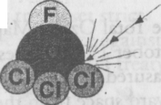
Starting in the early 1970’s, however, scientists have found evidence that human activities are disrupting the ozone balance. Human production of chlorine-containing chemicals such as chlorofluorocarbons (CFCs) has added an additional factor that destroys ozone. CFCs are compounds made up of chlorine, fluorine and carbon bound together. Because they are extremely stable molecules, CFCs do riot react easily with other chemicals in the lower atmosphere. One of the few forces that can break up CFC molecules is ultraviolet radiation. In the lower atmosphere, however, CFCs are protected from ultraviolet radiation by the ozone layer itself. CFC molecules thus are able to migrate intact up into the stratosphere. Although the CFC molecules are heavier than air, the mixing processes of the atmo­sphere carry them into the stratosphere.

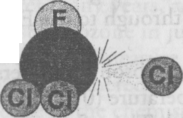
Once in the stratosphere, the CFC molecules no longer are shielded from ultraviolet radiation by the ozone layer. Bombarded by the sun’s ultraviolet energy, CFC molecules break up and release their chlo­rine atoms. The free chlorine atoms then can react with ozone molecules, taking one oxygen atom to form chlorine monoxide and leaving an ordinary oxygen molecule.

If each chlorine atom released from a CFC molecule destroyed only one ozone molecule, CFCs would pose very little threat to the ozone layer. However, when a chlorine monoxide molecule encounters a free

acorn of oxygen, the oxygen atom breaks up the chlorine monoxide, stealing the oxygen atom and releasing the chlorine atom back into the stratosphere to destroy more ozone. This reaction happens over and over again, allowing a single atom of chlorine to act as a catalyst, destroying many molecules of ozone.

Fortunately, chlorine atoms do not remain in the stratosphere forever. When a free chlorine atom reacts with gases such as methane (CH4), it is bound up into a molecule of hydrogen chloride (HC1), which can be carried downward from the stratosphere into the troposphere, where it can be washed away by rain. Therefore, if humans stop putting CFCs and other ozone-destroying chemicals into the stratosphere, the ozone layer eventually may repair its’elf.

Utraviolet radiation strikes a CFC

molecule..

...and causes a chlorine atom to break away.

Ozone Depletion

The term “ozone depletion” means more than just the natural destruction of ozone, it means that ozone loss is exceeding ozone creation. Think again of the “leaky bucket.” Putting additional ozone-destroying compounds such as CFCs into the atmosphere is like causing the “bucket” of ozone to spring extra leaks. The extra leaks cause ozone to leak out at a aster rate—faster than ozone is being created. Consequently, the level of ozone protecting us from ultraviolet radiation decreases.

The chlorine atom collides with an ozone molecule.

...and steals an oxygen atom to form chlorine monoxide, and leaves a molecule of ordinary oxygen.

In the area over Antarctica, there are stratospheric cloud and ice particles chat are not present at warmer latitudes. Reactions occur on the surface of the ice particles that accelerate the ozone destruction caused by stratospheric chlorine. This phenomenon has caused documented decreases in ozone concentrations over Antarctica. In fact, ozone levels drop so low in spring in the southern hemisphere that scientists have observed what they call a “hole” in the ozone layer.

When a free atom of

oxygen collides with the Chlorine monoxide...

In addition, scientists have observed declining concentrations of ozone over the whole globe. In the second half of 1993, for example, world wide ozone levels were the lowest ever recorded.

i

Monitoring Ozone from Space

...the two oxygen atoms form a molecule of oxygen.

The chlorine atom is thus released and free to destroy more ozone.

Since the 1920’s, ozone has been measured from the ground. Scientists place instruments at locations around the globe to measure the amount of ultraviolet radiation getting through the atmosphere at each site. From these measurements, they calculate the concentration of ozone in

the atmosphere above that location. These data, although useful in learning about ozone, are not able to provide an adequate picture of global ozone concentrations.

The Total Ozone Mapping Spectrometer (TOMS) instrument, first flown on the Nimbus-7 satellite in October 1978, makes daily, worldwide observations of the total amount of ozone in the atmosphere, measured on a Dobson scale (see next paragraph). TOMS measures sunlight that has been scattered back toward space from the atmosphere in multiple wavelengths. Since ozone absorbs ultraviolet light, the more ozone present, the less reflected ultraviolet radiation. To illustrate this principle, imagine pouring some water into a beaker and measuring the amount. Repeat the procedure, but now put a sponge between the glass and the beaker. Since the ozone acts like a sponge, absorbing the UV radiation, less gets through to the Earth’s surface and also less is reflected back out to space.

One Dobson unit refers to a layer of ozone that would be 0.001 cm thick under conditions of standard temperature (0°C) and standard pressure (1013.25 millibars, the average pressure at the surface of the Earth). Thus, for example, 300 Dobson units of ozone brought down to the surface of the Earth at 0°C would occupy a layer only 0.3 cm thick! When Dobson units fall below 225, a hole is said to exist (since there is actually still some ozone in the stratosphere, it is not a hole in the traditional sense, but the amount is not sufficient to prevent considerable harmful ultraviolet radiation from reaching the surface of the Earth). With less ozone to absorb harmful ultraviolet rays, more ultraviolet radiation is received at the surface of our planet. Amounts of ozone can be compared from region to region over vast areas by color coding the measurement units from the Dobson scale.

Contrary to the image created by the term “ozone layer,” the amount and distribution of Ozone mol­ecules in the stratosphere vary greatly over the globe. Ozone molecules are transported around the stratosphere much as water clouds are transported in the troposphere. Therefore, scientists observing ozone fluctuations over just one spot could not know whether a change in local ozone levels meant an alteration in global ozone levels, or simply a fluctuation in the concentration over that particular spot. Satellites have given scientists the ability to overcome this problem because they provide a picture of what is happening simultaneously over the entire Earth.

A continuing ozone monitoring program is underway using TOMS. TOMS instruments were flown on a Russian Meteor-3 polar-orbiting satellite in 1991 and on the Japanese Advanced Earth Observing Satellite-1 (ADEOS-1) in 1996. Additional TOMS instruments are scheduled to fly on several Earth Observing System (EOS) satellites in the future.

Scientists now are confident that stratospheric ozone is being depleted worldwide—partly due to human activities. However, scientists still do not know how much of the loss is the result of human activity, and how much is the result of fluctuations innatural cycles.

Predicting Ozone Levels

If scientists can separate the human and natural causes of ozone depletion, they can formulate improved models for predicting ozone levels. The predictions of early models already have been used by policy

makers to determine what can be done to reduce the ozone depletion caused by humans. For example, faced with the strong possibility that CFCs could cause serious damage to the ozone layer, policy makers from around the world in 1987 signed a treaty known as the Montreal Protocol. This treaty set strict limits on the production and use of CFCs. By 1990, the growing amount of scientific evidence against CFCs prompted diplomats to strengthen the requirements of the Montreal Protocol. The revised treaty called for a complete phaseout of CFC production in the developed countries by the year 1996.

However, scientists agree that much remains to be learned about the interactions that affect ozone. To create accurate models, scientists must study simultaneously all of the factors affecting ozone creation and destruction. Moreover, they must study these factors from space continuously, over many years, and over the entire globe. NASA’s Earth Observing System (EOS) will allow scientists to study ozone in just this way. The EOS series of satellites will carry a sophisticated group of instruments that will measure the interactions within the atmosphere that affect ozone. Building on the many years of data gathered by previous NASA missions, these measurements will increase dramatically our knowledge of the chemistry and dynamics of the upper atmosphere and our understanding of how human activities are affecting Earth’s protective ozone layer.

Seasonal Ozone Changes

Stratospheric ozone levels vary be season and latitude. Since 1979, mid-latitude (30° - 60°) ozone levels have fallen about 5%. The creation of the ozone hole involves high concentrations of chlorine, polar stratospheric clouds, and a strong wind vortex (called the polar vortex). Ozone loss is accelerated over Antarctica because the stratosphere contains icy particles which make it difficult for chlorine and bromine to be included in “safe molecular forms” and increase their role as destructive chemicals that can break apart ozone molecules with amazing efficiency. During the polar night, when several months of darkness descend on Antarctica, temperatures plummet below -80°C. The real action begins when the Sun returns to this part of the world during springtime, energizing the chemical cycle that destroys ozone.

Exposure Category	Index Value	Precautions
lyfinimal	0-2	hat
Low	3-4	sunscreen (15+)
Moderate	5-6	shady areas
High	7-9	indoors 10 AM-4 PM
Very High	10+ ~	indoors all day

Health Effects of Ultraviolet Radiation

We also measure the amount of ultraviolet radiation reaching the surface. Ultraviolet light, especially UV-B, can be dangerous. It can cause immediate effects such as blistering sunburns, as well as longer- term problems like skin cancer and cataracts. Higher levels can suppress the immune system, and lower phytoplankton populations (phytoplankton comprise the bottom of the marine food web). For each 1% decrease in stratospheric ozone there is calculated to be a 2% increase in the amount of solar ultraviolet radiation reaching the ground. This could raise the number of skin cancer cases by 3% to 6% per year.

In 1994, the National Weather Service and the Environmental Protection Agency developed the Ultraviolet (UV) Index as a way of quantifying the amount of exposure to ultraviolet radiation for a specific day. The index numbers range from 0 to 10+. In conjunction with the UV Index, the EPA has initiated a toll-free Stratospheric Ozone Information Hotline (1-800-296-1996). Callers can request information on how the United States is implementing stratospheric ozone policy.

Clouds and the Energy Cycle

The study of clouds, where they occur, and their characteristics, may well be a central key to understand­ing climate change. Low, thick clouds primarily reflect solar radiation and cool the surface of the Earth. High, thin clouds primarily transmit incoming solar radiation; at the same time, they trap some of the outgoing infrared radiation emitted by the Earth and radiate it back downward, thereby warming the surface of the Earth.

Whether a given cloud will heat or cool the surface depends on several factors, including the cloud’s altitude, its size, and the make-up of the particles that form the cloud. The balance between the cooling and warming actions of clouds is very close although, overall, averaging the effects of all the clouds around the globe, cooling predominates.

The Earth’s climate system constantly adjusts in a way that tends toward maintaining a balance between the energy that reaches the Earth from the sun and the energy that goes from Earth back out to space. Scientists refer to this as Earth’s “radiation budget.” The components of the Earth system that are important to the radiation budget are the planet’s surface, atmosphere, and clouds. The energy coming from the sun to the Earth’s surface is called solar energy. Most of it is in the form of radiation from the “visible” wavelengths, i.e., those responsible for the light detected by our eyes. Visible radiation and radiation with shorter wavelengths, such as ultraviolet radiation are labeled “shortwave.” Both the amount of energy and the wavelengths at which energy is emitted by any system are controlled by the average temperature of the system’s radiating surfaces, plus the emission properties. The temperature of the sun’s radiating surface, or photosphere, is more than 5500°C (9900°F). However, not all of the sun’s energy comes to Earth. The sun’s energy is emitted in all directions, with only a small fraction being in the direction of the Earth.

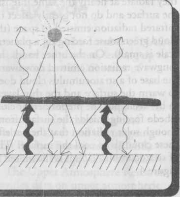
Energy goes back to space from the Earth system in two ways: reflection and emission. Part of the solar energy that comes to Earth is reflected back out to space in the same, short wavelengths in which it came to Earth. The fraction of solar energy that is reflected back to space is called the albedo. Different parts of the Earth have different albedos. For example, ocean surfaces and rain forests have low albedos, which means that they reflect only a small portion of the sun’s energy. Deserts, ice, and clouds, how­ever, have high albedos; they reflect a large portion of the sun’s energy. Over the whole surface of the Earth, about 30 percent of incoming solar energy is reflected back to space. Because a cloud usually has a higher albedo than the surface beneath it, the cloud reflects more shortwave radiation back to space than the surface would in the absence of the cloud, thus leaving less solar energy available to heat the surface and atmosphere. Hence, this “cloud albedo forcing,” taken by itself, tends to cause a cooling or “negative forcing” of the Earth’s climate. The shortwave reflection by clouds is illustrated in Figure 1.

Another part of the energy going to space from the Earth is the electromagnetic radiation emitted by the Earth. The solar radiation absorbed by the Earth causes the planet to heat up until it is emitting as much energy back into space as it absorbs from the sun. Because the Earth is absorbing only a tiny fraction of the sun’s energy, it remains cooler than the sun, and therefore emits much less radiation.

Most of this radiation is at longer wavelengths than solar radiation. Unlike solar radiation, which is

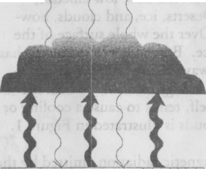
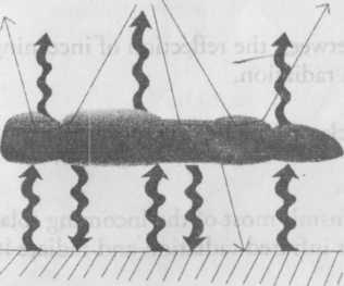
Figure 2. Longwave rays emitted by the Earth are absorbed and reemitted by a cloud, with some rays going to space and some going to the surface. Wavy arrows indicate longwave rays (distinguishedfrom straight arrows, which indicate shortwave rays, as in the previous figure), and thicker arrows indicate more energy. The resulting "cloud greenhouse forcing, ” taken by itself, tends to cause a warming of the Earth.

mostly at wavelengths visible to the human eye, the Earth’s longwave radiation is mostly at infrared wavelengths, which are invisible to the human eye. When a cloud absorbs longwave radiation emitted by the Earth’s surface, the cloud reemits a portion of the energy to outer space and a portion back toward the surface. The intensity of the emission from a cloud varies directly as its temperature and also depends upon several other factors, such as the cloud’s thickness and the makeup of the particles that form the cloud. The top of the cloud is usually colder than the Earth’s surface. Hence, if a cloud is introduced into a previously clear

sky, the cold cloud top will reduce the longwave emission to space, and (disregarding the cloud albedo forcing for the moment) energy will be trapped beneath the cloud top. This trapped energy will increase the temperature of the Earth’s surface and atmosphere until the longwave emission to space once again balances the incoming absorbed shortwave radiation. This process is called “cloud greenhouse forcing” and, taken by itself, tends to cause a heating or “positive forcing” of the Earth’s climate. Usually, the higher a cloud is in the atmosphere, the colder is its upper surface and the greater is its cloud greenhouse forcing. The absorption and reemission of longwave radiation by clouds is illustrated in Figure 2.

If the Earth had no atmosphere, a surface temperature ar below freezing would produce enough emitted radiation to balance the absorbed solar energy. But the atmosphere warms the planet and makes Earth more livable. Clear air is largely transparent to incoming shortwave solar radiation and, hence, transmits

it to the Earth’s surface. However, a signifi cant fraction of the longwave radiation emitted by the surface is absorbed by trace gases in the air. This heats the air and causes it to radiate energy both out to space and back toward the Earth’s surface. The energy emitted back to the surface causes it to heat up more, which then results in greater emission from the surface. This heating effect of air on the surface, called the atmospheric greenhouse effect, is due mainly to water vapor in the air, but also is enhanced by carbon dioxide, methane, and other infrared-absorbing trace gases.

In addition to the warming effect of clear air, clouds in the atmosphere help to moder- ate the Earth’s temperature. The balance of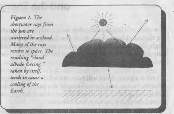

the opposing cloud albedo and cloud green­house forcings determines whether a certain cloud type will add to the air’s natural warming of the Earth’s surface or produce a cooling effect. As explained below, the high thin cirrus clouds tend to enhance the heating effect, and low thick stratocumulus clouds have the opposite effect, while deep convective clouds are neutral. The overall effect of all clouds together is that the Earth’s surface is cooler than it would be if the atmosphere had no clouds.

High Clouds

Figure 3. Cirrus clouds transmit most of the incoming shortwave radiation, but they trap some of the outgoing longwhve radiation. Their cloud greenhouse forcing is greater than their albedo forcing, resulting in a net warming of the Earth.

The high, thin cirrus clouds in the Earth’s atmosphere act in a way similar to clear air because they are highly transparent to shortwave radiation (their cloud albedo forcing is small), but they readily absorb the outgoing longwave radiation. Like clear air, cirrus clouds absorb the Earth’s radiation and then emit longwave, infrared radiation both out to space and back to the Earth’s surface. Because cirrus clouds are high, and therefore cold, the energy radiated to outer space is lower than it would be without the cloud (the cloud greenhouse forcing is large). The portion of the radiation thus trapped and sent back to the Earth’s surface adds to the shortwave energy from the sun and the longwave energy from the air already reaching the surface. The additional energy causes a warming of the surface and atmosphere. The overall effect of the high thin cirrus clouds then is to enhance atmospheric greenhouse warming. The effect of cirrus clouds is illus­trated in Figure 3.

Low Clouds

Figure 4. Stratocumulus clouds reflect much of the incoming shortwave radiation but also reemit large amounts of longwave radiation. Their cloud albedo forcing is larger than their cloud greenhouse forcing, resulting in a net cooling of the Earth.

In contrast to the warming effect of the higher clouds, low stratocumulus clouds act to cool the Earth system. Because lower clouds are much thicker than high cirrus clouds, they are not as transparent: they do not let as much solar energy reach the Earth’s surface. Instead, they reflect much of the solar energy back to space (their cloud albedo forcing is large). Although stratocumulus clouds also emit longwave radiation out to space and toward the Earth’s surface, they are near the surface and at almost the same temperature as the surface. Thus,

Clouds

they radiate at nearly the same intensity as the surface and do not greatly affect the infrared radiation emitted to space (their cloud greenhouse forcing on a planetary scale is small). On the other hand, the longwave radiation emitted downward from the base of a stratocumulus cloud does tend to warm the surface and the thin layer of air in between, but the preponderant cloud albedo forcing shields the surface from enough solar radiation that the net effect of these clouds is to cool the surface. The effect of stratocumulus clouds is illustrated in Figure 4.

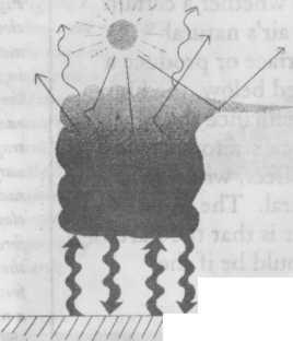
Figure 5. Deep convective clouds emit little longwave radiation at the top but much at the bottom. They also reflect much of the incoming shortwave radiation. Their cloud greenhouse and albedo forcings are both large, but nearly in balance, resulting in neither warming nor cooling.

Deep Convective Clouds

In contrast to both of the cloud categories previously discussed are deep convective clouds, typified by cumulonimbus clouds. A cumulonimbus cloud can be many kilometers thick, with a base near the Earth’s surface and a top frequently reaching an altitude of 10 km (33,000 feet), and sometimes much higher. Because cumulonimbus cloud tops are high and cold, the energy radiated to outer space is lower than it would be without the cloud (the cloud greenhouse forcing is large). But because they also are very thick, they reflect much of the solar energy back to space (their cloud albedo forcing is also large); hence, with the reduced shortwave radiation to be absorbed, there is essentially no excess radiation to be trapped. As a consequence, overall, the cloud greenhouse and albedo forcings almost balance, and the overall effect of cumulonimbus clouds is neutral—neither warming nor cooling. The effect of deep convective clouds is illustrated in Figure 5.

Clouds—A Key Variable in Global Change

• The effect of clouds on climate depends on the competition between the reflection of incoming solar radiation and the absorption of Earth’s outgoing infrared radiation.

• Low clouds have a cooling effect because they are optically thick and reflect much of the incom­ing solar radiation out to space.

• High thin cirrus clouds have a warming effect because they transmit most of the incoming solar radiation while, at the same time, they trap some of the Earth’s infrared radiation and radiate it back to the surface.

• Deep convective clouds, on average have neither a warming nor a cooling effect because their cloud greenhouse and albedo forcings, although both large, nearly cancel one another.

NASA Missions to Study Clouds and the Energy Cycle

Studies of clouds and the energy cycle have been performed for many years as part of a number of NASA missions. In the near future, small missions addressing specific investigations are planned, leading up to the main initiative of NASA’s Earth Science Program, the Earth Observing System (EOS) series of satellites beginning in 1999.

Historically, the Television Infrared Observation Satellite (TIROS) series provided a technology test to obtain daily temperature and global cloud-cover data. The Nimbus series provided the first global radiation budget analysis from space, indicating that the planetary albedo was lower and the outgoing infrared radiation higher than previously believed. The Earth Radiation Budget Experiment (ERBE) provided an improved and more-comprehensive analysis of the global radiation budget and, especially, the first global observations of cloud greenhouse and albedo forcings. The Upper Atmosphere Research Satellite (UARS) monitors the solar energy reaching the Earth and provides data on upper atmospheric chemistry and dynamics. The early Spacelab/Space Transportation System (STS) and the Atmospheric Laboratory for Applications and Science (ATLAS) payloads launched on the Space Shuttle provided data on solar energy, sun-atmosphere interactions, and upper atmospheric chemistry and dynamics.

The Next Steps

An important mission for the study of clouds is the joint U.S./Japan Tropical Rainfall Measuring Mis­sion (TRMM). TRMM, launched in November 1997 carries the EOS Clouds and the Earth’s Radiant Energy System (CERES) instrument, an improved version of the ERBE instrumentation. Also, TRMM carries instrumentation to study evaporation of water vapor into the atmosphere and its condensation to produce rainfall, processes of primary importance to the global energy budget. Several of the EOS series of satellites will carry the CERES instrument and other advanced instrumentation to provide a highly- accurate, self-consistent, and long-term (15 years) cloud and radiation data base. Analyses of these data, building on the foundation laid by previous missions, will lead to a better understanding of the role of clouds and the energy cycle in global climate change.

Volcanoes

Volcanoes and Global Cooling

Volcanic gases are thought to be responsible for the global cooling that has sometimes been observed for a few years after a major eruption. Recent studies have shown that when sulfate aerosols released by volcanic eruptions reach the stratosphere, they can produce a large, widespread cooling effect. The aerosols reflect a great deal of incoming solar radiation back out to space and therefore create a net cooling effect on the surface of the Earth. In fact 1992, following the eruption of Mt. Pinatubo in June 1991, was one of the coolest years on record.

The dispersal of aerosols depends on the amount ejected, the angle and strength of ejection, and the latitude of occurrence. If the volcano ejects the material out of its side, then most of the sulfur dioxide will stay in the troposphere and will not be widely dispersed. However, if the material is ejected vertically and enters the stratosphere, there are increased chances that the aerosols will be widely distributed by the prevailing wind belts of our planet. Less mixing occurs between the high latitiude wind belts and the rest of the planet, especially during the polar winters, and therefore, volcanoes that erupt in high latitudes (60°+) are less likely to have global effects. The opposite is true of mid . '" and low latitude eruptions because there is a W great amount of mixing between them.

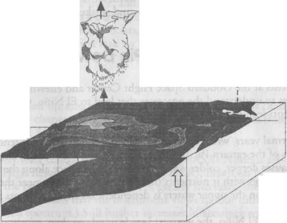
Figure 1. Volcanism studies are an important aspect of climate research.

Mt. Pinatubo, erupted on June 15, 1991.

Located in the Philippines at 15.0 °N and 120.0°E, the aerosol cloud travelled westward with the prevailing winds.

More than 5 billion cubic meters of ash and pyroclastic debris were ejected from the volcano. The eruption caused 847 deaths, 184 injuries, and displaced approximately 1 million people.

Figure 1 illustrates that as volcanoes erupt, they blast huge clouds into the atmosphere. These clouds are made up of particles and gases, including sulfur dioxide. Millions of tons of sulfur dioxide gas can reach the strato­sphere from a major eruption.

There, the sulfur dioxide converts to tiny persistent sulfuric acid

(sulfate) particles, referred to as

aerosols. These sulfare particles reflect energy coming from sun, thereby decreasing the amount of sunlight reaching and heating the Earth’s surface.

Short term global cooling often has been linked with some major volcanic eruptions. The year 1816 has been referred to as “the year without a summer.” It was a time of significant weather-related disruption in New England and in Western Europe with killing summer frosts in the United States and Canada. These strange phenomena were attributed to a major eruption of the Tambora volcano in 1815 in Indonesia. The volcano threw sulfur dioxide gas into the stratosphere, and the aerosol layer that formed led to brilliant sunsets seen around the world for several years.

But, not all volcanic eruptions, not even all large volcanic eruptions, produce global-scale cooling.

Mount Agung in 1963 apparently caused a considerable decrease in temperatures around much of the world, whereas El Chichon in 1982 seemed to have little effect, perhaps because of its different location or because of the El Nino that occurred the same year. (See El Nino chapter.) El Nino is a Pacific Ocean phenomenon, but it causes worldwide weather variations that may have acted to cancel out the effect of the El Chichon eruption.

Volcanoes and Ozone Depletion

Another possible effect of a volcanic eruption is the destruction of stratospheric ozone. Researchers now are suggesting that aerosol particles containing sulfuric acid from volcanic emissions may contribute to ozone loss. When chlorine compounds resulting from the breakup of chlorofluorocarbons (CFCs) in the stratosphere are present, the sulfate particles may serve to convert them into more-active forms that may cause more-rapid ozone depletion. (See Ozone chapter.)

Monitoring the Effects of Volcanoes

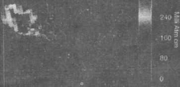
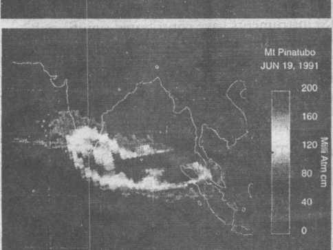
Space-based instruments are the only practical way to observe large and transitory volcanic eruption clouds. NASA’s Total Ozone Mapping Spectrometer (TOMS) instruments have contributed significantly to our knowledge of the total amount of sulfur dioxide emitted into the atmosphere in the course of major volcanic eruptions. Figure 2 shows TOMS images of sulfur dioxide spreading across the Indian Ocean region following the eruption of Mount Pinatubo. Several weeks later the sulfur dioxide had spread around the world as observed by the Microwave Limb Sounder (MLS) instrument on NASA’s Upper Atmosphere Research Satellite (UARS) (Figure 3).

In addition to detecting the sulfur dioxide from Mount Pinatubo, TOMS has made similar observations of more than 100 volcanic events, including a major eruption from the Cerro Hudson volcano in Chile in 1991. TOMS instruments were launched on a Nimbus-7 spacecraft in 1978; a Russian Meteor-3 spacecraft in 1991; and on the Earth Probe and the Japanese Advanced Earth Observing System (ADEOS) platforms in 1996. ATOMS instrument is also scheduled to fly on a Russian-3M satellite in 2000.

Data from the Stratospheric Aerosol and Gas Experiment (SAGE II) instrument on NASA’s Earth Radiation Budget Satellite (ERBS) have shown that during the first five months after the Mount

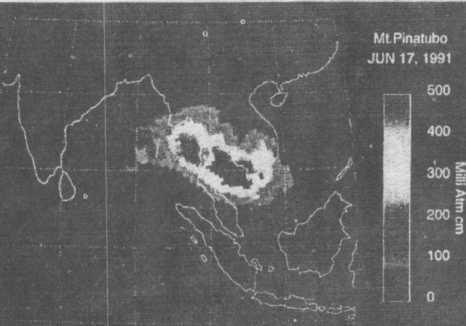
Sulfur Dioxide NIMBUS-7 TOMS NflSVGSFC

* • 400

!" 320

. Sulfur Dioxide NIMBUS-7 TOMS (WVS/YGSFC

Sulfur Dioxide NIMBUS-7 TOMS „ ftlAS/VGSFC

О

Mi Pinatubo JUN 18. 19У1

Figure 2: Images from Nimbus -7 TOMS showing the spread of sulfur dioxide from the Mt. Pinatubo eruption. The “gray scale" indicates the thickness of the sulfur dioxide layer would have if observed at standard surface conditions of temperature and pressure.

Pinatubo eruption, the optical depth of the strato­spheric aerosol increased up to 100 times in certain locations. Optical depth is a general measure of the capacity of a region of the atmo­sphere to prevent the passage of visible light through it. Greater optical depths mean greater blockage of the light. In this case, the increased optical depth means that considerably less of the sun’s energy can get through the cloud to warm the Earth’s surface. An advanced SAGE III instru­ment, which will make similar observations, is scheduled to be launched on a Russian Meteor- 3M spacecraft in the second half of 1998.

Observations of the effects of Mt. Pinatubo aerosols on global climate have been used to validate scientists’ understanding of climate change and our ability to predict future climate. Research­ers at NASA’s Goddard Institute for Space Studies in New York city have applied their general circu­lation model of Earth’s climate to the problem. They have reported success in correctly predicting many of the effects of the sulfate aerosols from Mount Pinatubo’s eruption on lowering global temperatures.

NASA Missions to Study Volcanoes

Some of NASA’s past and present missions that contribute to the study of volcanoes are listed in the accompanying table. Included in the table is the Earth Observing System (EOS), the key element of NASA’s Earth Science Enterprise. The first launch in the series of EOS satellites is sched­uled to take place in 1998.

Figure 3. Images from the UARS satellite—sulfur dioxide cloud from Mt. Pinatubo on September 23, 1991, after dispersal around the world

The High Resolution Infrared Radiometer (HRIR), first flown on NASA’s Nimbus-1 satellite in 1964, has been used to observe both active and dormant volcanoes. On Nimbus-2, HRIR recorded energy changes from the volcanic activity on Surtsey, Iceland in 1966. The Multispectral Scanner (MSS) and Thematic Mapper (TM) instruments on the Landsat satellites have provided a long series of images of volcanic activity, such as venting, volcanic ash falls, and lava flows.

The EOS program will incorporate a series of satellites that will carry advanced instruments to provide a highly-accurate, self-consistent, and long-term data base of many aspects of Earths atmosphere, land, and ocean characteristics. The information gained from this major effort to study Earth phenomena will expand our knowledge of the interactions of volcanoes with Earth’s climate.

Glossary of Chemistry

Cl,	chlorine molecule
HC1	hydrogen chloride
н,о	water
°3	ozone
	sulfuric acid
SO,	sulfur dioxide

The Child

Fishermen who ply the waters of the Pacific off the coast of Peru and Ecuador have known for centuries about the El Nino. Every three to five years during the months of December and January, fish in the coastal waters off of these countries virtually vanish, causing the fishing business to come to a standstill. South American fishermen have given this phenomenon the name El Nino, which is Spanish for “The Child,” because it comes about the time of the celebration of the birth of the Christ Child.

An understanding of the complex processes at work to produce the El Nino requires information about phenomena occurring all across the tropical Pacific,: not just its eastern boundary, the west coast of South America. Remote sensing, particularly from the weather satellites, has been the source of data that finally has made it possible to understand the interactions between atmospheric winds and oceanic tempera­tures and currents that lead to the El Nino.

Worldwide Effects

Warm Surface Temperature

The cycle of El Nifio is com­pleted as the weakened trade winds allow eastward currents to flow, carrying warm water from the western Pacific, and reinforcing the original warm­ing trend.

Eastward

Currents

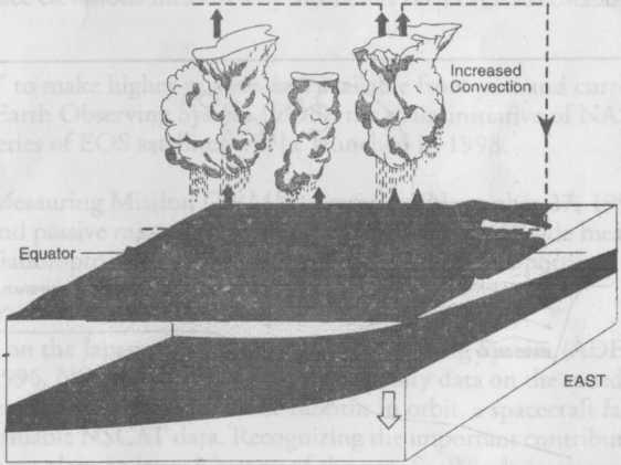
Increased

Convection

Weakened Trade Winds

bird populations on islands in the Pacific; flooding and landslides in Peru, Ecuador and in the Colorado River basin of the United States; 6 tropical cyclones in Tahiti; devastation of coral reefs throughout the Pacific; and drought, disease, and malnutrition in South Africa.

Nightly cloud images on weather satellites show us the that cross the Pacific and travel regions to the central lands of indirect or secondary El Nino eflocations worldwide. During the 1982 drought-related fires in Borneo and Aus-

El Nino effects are not limited to Ecuador. They can be transmitparts of the world, the disruphave tragic and/or profound Nino has been shown to be flooding in Texas in the to the anomalous warmth east United States in the

television news from paths followed by the storms northward from equatorial North America. Important fects have been noted in other 1983 El Nino, there were huge tralia; drought-related eradication of sea

the disturbed areas off of Peru and ted great distances. In many tion of normal climate can economic consequences. El related to the unusual winter of 1991-1992 and experienced in the south- same period.

Closer to home El Nino years have been associated with changing North Pacific atmospheric and oceanic currents bringing warmer waters to the west coast of Washington, Oregon, and Callifornia. These changes have been responsible for increased shark attacks off the Oregon coast, increased spinal injuries

in California (due to weather- altered coastal sea floors that fooled surfers), and changes in salmon populations. In addition, the east coast of the United States has experienced warmer and wetter springtime conditions, increasing the mosquito popula­tion and encephalitis cases. Changing weather patterns have driven mice, and therefore snakes into Montana, increasing snake bite incidents. Cooler and wetter springtime conditions in New Mexico have led to a rise in bubonic plague as the rodent population increased.

Air/Sea Interaction

Normal Conditions

WEST

Convective Loop

Equator

1 До i

Figure 1. Normal conditions over the Pacific basin

A key element of the El Nino phenomenon is the interaction between the winds in the atmo­sphere and the sea surface. With­out this air/sea interaction, there would be no El Nino. Taking advantage of observations from the National Oceanic and Atmo­spheric Administration (NOAA) weather satellites, scientists have been able to track shifting pat­terns of sea surface temperatures. The pool of warm waters that normally resides in the western waters of the Pacific has been seen to drift eastward toward the western coast of South America.

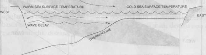
El Nifio Conditions

WEST

Figure 2. Disturbed conditions over the Pacific basin during an El Nino.

T his foretells the advent of an El Nino.

NASA satellite images also help us see the shifting patterns of storms over the equator that are a conse­quence of the shifting locations of

the warm water pool. Towering cumulus clouds, reaching high into the atmosphere with multiple regions of strong up- and- down vertical (convective) motions, form and move eastward across the Pacific as they are generated by the warm surface waters. This movement of the powerfully active convec­tive regions alters the surface winds, and weakens the normally prevailing east-to-west trade winds. (See Figures 1 and 2.)

Space Observations Pin Down the El Nino Phenomenon

Scientists at the Goddard Space Flight Center and elsewhere have used numerical models and theoretical studies to understand the processes that lead to El Nino. Comparison with data has shown the sequence of events leading up to El Nino.

In normal years, when there is no El Nino, the trade winds tend to blow from east to west across the waters of the eastern Pacific. They tend to drag the surface waters westward across the ocean. In turn, this causes deeper, colder waters to rise to the surface along the coast. The “upwelling” of deep ocean waters brings with it nutrients that otherwise would lie near the bottom of the ocean. The fish popula­tion living in the upper waters is dependent on these nutrients from below for survival.

During an El Nino, the westward trade winds weaken, causing the upwelling of deep water to cease. The consequent warming of the ocean surface further weakens the trade winds, and strengthens El Nino. Without upwelling, the nutrients from the deep water are no longer available. This signals a severe reduction in the fishing industry until the time that normal conditions return.

Prediction of El Nino events is now the focus of a major scientific initiative. The prediction of El Nino requires sophisticated numerical models to simulate: 1) the changes within the ocean that cause surface

Schematic of the main pro­cesses thought to produce El Nino. Above-normal sea sur­face temperatures produce in­creased precipitation and changes in atmospheric circulation. These tend to maintain the warm temperatures by driving oceanic currents. Some of these effects are immediate; others act after the forced signal reflects from the western boundary and returns to the region of strong cou- pling.

WEAK	STRONG	WEAK
COUPLING	COUPLING	COUPLING

.

temperatures to warm; 2) the changes in atmospheric convection and clouds due to surface warming; and 3) the changes in surface winds that are caused by the convective disturbances. The societal impacts of accurately forecasting El Nino up to a year in advance are huge, allowing economic and agricultural policy makers to adapt to short-term climate fluctuations in a beneficial way. Satellite observations will continue to play a crucial role in ensuring the success of these forecasts, by providing accurate measure­ments of the present conditions in the region, an essential first task for prediction.

NASA Missions to Study El Nino

Over the years, several NASA missions have studied the effects associated with El Nino, such as changes in sea-surface temperature (SST) and cloud cover changes. These studies are augmented by data from operational satellites of the National Oceanic and Atmospheric Administration (NOAA).

Initial efforts at mapping SST and cloud cover were conducted using data from NASA’s Nimbus series of satellites. The four-channel Advanced Very High Resolution Radiometer (AVHRR), flown on NOAA’s TIROS-N weather satellite in 1978 and on the NOAA-6 satellite in 1979, greatly increased the accurate measurements of El Nino effects. (“Four channel” means that the instrument views in four different parts of the electromagnetic visible and infrared spectrum.) Still further increases in accuracy resulted when a fifth channel was added to the AVHRR instrument flown on NOAA-7 in 1981, and on subse­quent NOAA satellites. The fifth channel improved the measurement of SST by providing corrections for atmospheric water vapor that otherwise would have interfered with the temperature measurements.

The joint U.S.-French TOPEX/Poseidon mission was launched in 1992 and is providing global determi­nations of changes in ocean surface currents that are related to the El Nino phenomenon. The currents are determined from changes in ocean surface elevations measured by altimeters on TOPEX/Poseidon with accuracies of a few centimeters.

NASA has initiated a “Pathfinder Program” to make higher-quality data available from past and current missions. These efforts will lead up to the Earth Observing System (EOS), the main initiative of NASA’s Earth Science Enterprise. The first in the series of EOS satellites will be launched in 1998.

The joint U.S.-Japanese Tropical Rainfall Measuring Mission (TRMM), launched November 27, 1997 uses for the first time, both active (radar) and passive microwave detectors from space to provide mea­surements of precipitation, clouds, and radiation processes in lower latitudes, including the portions of the Pacific Ocean where El Nino occurs.

A NASA scatterometer called NSCAT flew on the Japanese Advanced Earth Observing System (ADEOS) spacecraft, which was launched in August 1996. NSCAT provided very high quality data on the speed and direction of ocean-surface winds worldwide. Unfortunately, after nine months in orbit, a spacecraft failure brought to an end the stream of extremely valuable NSCAT data. Recognizing the important contributions to Earth science made by NSCAT, NASA now plans to launch a copy of the new SeaWinds scatterometer as early as November 1998 as part of a dedicated mission named QuikSCAT to bridge the gap remaining before launch (planned for August 1999) of the Japanese spacecraft designated ADEOS II, which will also carry a SeaWinds instrument.

In addition to the scatterometer measurements, which use active microwave radar systems to determine surface wind speeds and directions over the ocean, surface wind speeds are also being obtained from a passive microwave sensor on a Department of Defense spacecraft. The instrument is called the Special Sensor Microwave/Imager (SSM/I).

Key sources of Pathfinder data related to El Nino are data from the five-channel AVHRRs flown on NOAA- 7, 9, and 11. These historic data sets cover the period 1981 through 1992 and beyond and will permit more-accurate SST determinations than were previously available. These data are important to the devel­opment and testing of a new generation of computer models in which the interacting processes of the land, the atmosphere, and the oceans are coupled. These coupled models will lead the way to an increased understanding of phenomena such as El Nino and the teleconnections that link El Nino with changes in weather patterns throughout the world.

NASA’s SeaWiFS (Sea-viewing Wide Field of View Sensor) was launched on the Orb View-2 satellite in August 1997. The SeaWiFS sensor is designed to detect ocean color, which is an indicator of microscopic plant life in the ocean. The growth of such plants (called phytoplankton) is affected by the changes in sea surface temperature that are related to El Nino.

With the launch of the EOS satellites, starting in 1999, we will have the means to collect and analyze the most-comprehensive data set ever acquired for the development of coupled models. This data set will increase markedly our understanding of the causes and effects of such large-scale ocean-atmosphere phenomena as El Nino.

significantly over periods of days or months. Each of these factors contributes differently to sea level height. Their respective impacts can be:

• Ocean eddies-up to about 25 centimeters (10 inches)

• Temperature of the upper ocean water—up to about 35 centimeters (13 inches), similar to the contribution from ocean eddies

• Tides in the deep ocean up to 1 meter (3 feet)

• Ocean currents or ocean circulation-about 2 meters (6 feet)

• Gravity - up to 150 meters! (almost 500 feet!)

Believe it or not, the height of the Earths oceans changes by approximately 150 meters (almost 500 feet) between the north Indian Ocean (off of the south coast of India) and the western Pacific Ocean (off New Guinea)! Earth’s geoid is a calculated surface of equal gravitational potential energy and represents the shape the sea surface would have if the ocean were not in motion. How the “real” ocean surface differs from the geoid gives ocean currents. To study how various factors like ocean circulation and eddies affect the height of our oceans, oceanographers eliminate the height of sea surface caused by gravity.

How the Earth's rotation affects winds and currents

Our planet’s rotation produces an apparent force on all bodies moving relative to the Earth. This force is greatest at the poles and least at the Equator because of Earth’s approximately spherical shape; i.e., the apparent force, called the Coriolis effect increases with increasing latitude. The Coriolis effect, causes the direction of winds and ocean currents to be deflected. The “rule of thumb” is that in the Northern Hemisphere, wind and currents are deflected to the right; in the Southern Hemisphere they are deflected to the left. You can better imagine how the Coriolis effect works with the use of a turntable, a round piece of cardboard, a ruler, and a marker. Place the cardboard on the turntable and spin it counterclockwise (emulating the Northern Hemisphere). Hold the ruler still and draw a straight line on the cardboard from the center (the North Pole) to the edge (the equator). Even though you draw a straight line, the line on the moving cardboard is curved to the right. Also, try spinning the turntable in a clockwise direction (emulating the Southern Hemisphere) and at different speeds. You will notice that your line is curved to the left and that the faster you spin the turntable, the more curved the line is.

Hills and Valleys in the Ocean

The direction of ocean currents at the sea surface is related to wind forcing. However, the Coriolis effect also affects the motion of the ocean. The “Coriolis effect” causes the movement of water in the uppermost wind-driven part of ocean (known as the “Ekman layer”) to create hills and valleys in the ocean topography, or shape. In the Northern Hemisphere, counterclockwise winds cause surface ocean water to move to the tight and away from a central point, causing a sea surface valley. The slope of the sea surface creates currents that flow around these hills and valleys, known as “geostrophic currents.” In the Northern Hemisphere, clockwise-flowing winds cause surface ocean water to move to the right and toward a the central point, causing a sea surface hill. “Geostrophic currents” flow around these high and low centers of water pressure, similar to how winds blow from high to low pressure. They are located below the wind- driven layer and their velocity is proportional to the slope of the sea surface. These “hills” and “valleys”— or ocean topography—are measured by TOPEX/Poseidon and used to calculate “geostrophic” ocean currents, similarly to how meteorologists use atmospheric pressure maps to track winds and weather.

Dynamic Ocean Topography - Sea Level Height Changes for the Long Run

Ocean currents are mapped by studying the “hills” and “valleys” in maps of the height of the sea surface relative to the geoid. This height is called “Dynamic Ocean Topography.” Currents move around ocean dynamic topography “hills” and “valleys” in a predictable way. Note that a clockwise sense of rotation is found around “hills” in the Northern Hemisphere and “valleys” in the Southern Hemisphere. This is because of the Coriolis effect. Conversely, a counterclockwise sense of rotation is found around “valleys” in the Northern Hemisphere and “hills” in the Southern Hemisphere. In general, major ocean currents are stable and so maps of dynamic ocean topography change very little over time.

Changes in Sea Height Over Short Time Scales

Just like the atmosphere, the oceans have seasons. In a similar fashion to the way air temperatures change with the seasons, ocean temperatures change on a “seasonal” basis too. During the summer months, surface ocean temperatures increase, causing a rise in sea heights. Conversely, during the winter months when ocean temperatures decrease, there is a decrease in sea heights. In the Northern Hemisphere, the overall change in sea surface height between these seasons is very dramatic, while in the Southern Hemisphere, season-to-season changes are much more moderate. The “ocean seasons” look different in the

Northern and Southern Hemispheres because the oceans have a slower reaction to seasonal temperature differences than land surfaces have and there is a higher percentage of ocean in the Southern Hemisphere than in the Northern Hemisphere. Comparatively, sea surface variability due to the ocean seasons is about 1/16 of the overall variation in sea surface height caused by ocean circulation (dynamic ocean topography). Sea surface variability maps are used to study the changes in sea height over months or seasons. They show how currents vary over short times and distances as well as showing seasonal changes in the temperature of the upper ocean layer.

NASA's Mission to Study Ocean Topography

In August 1992, TOPEX/Poseidon (named after the Greek God of the oceans) was launched into low Earth orbit by an Ariane 42P rocket from the European Space Agency’s Space Center located in Kourou, French Guiana—the first launch of a NASA payload from this site. From its orbir 1,336 kilometers (830

miles) above the Earth’s surface, TOPEX/Poseidon measures sea level along the same path every 10 days using a dual frequency altimeter developed by NASA and a CNES single frequency solid-state altimeter. This information is used to relate changes in ocean currents with atmospheric and climate patterns. Measurements from NASA’s Microwave Radiometer provide estimates of the total water-vapor content in the atmosphere, which is used to correct errors in the altimeter measurements. These combined measurements allow scientists to chart the height of the seas across ocean basins with an accuracy of less than 13 centimeters (5 inches)!

TOPEX/Poseidon is a vital part of a strategic research effort to explore ocean circulation and its interaction with the atmosphere. It complements a number of international oceanographic and meteorological programs, including the World Circulation Experiment (WOCE) and the Tropical Ocean and Global Atmosphere (TOGA) Program, both of which are sponsored by the World Climate Research Program (WCRP). TOPEX/Poseidon’s three-year prime mission ended in fall 1995 and is now in its extended observational phase. Its first follow-on mission, Jason-1, will continue this program of long-term observations of ocean circulation from space into the next century.

Information courtesy of the Jet Propulsion Laboratory (JPL), Pasadena, CA. Additional information can be found at http://topex-www.jpl.nasa.gov/education/tutoriall.html

Polar lce

Polar ice consists of sea ice formed from the freezing of sea water, and ice sheets and glaciers formed from the accumulation and compaction of falling snow. Both types of ice extend over vast areas of the polar regions. Global sea-ice coverage averages approximately 25 million km2, the area of the North American continent, whereas ice sheets and glaciers cover approximately 15 million km2, roughly 10% of the Earth’s land surface area.

Effects on Energy Exchange

\

Ice, both on land and in the sea, affects the exchange of energy continuously taking place at the Earth’s surface. Ice and snow are among the most reflective of naturally occurring Earth surfaces. In particular, sea ice is much more refjective than the surrounding ocean, so that if it were to increase in extent, for instance because of large-scale cooling, then more solar energy would be reflected back to space and less would be absorbed at the surface. This would tend to cool the local region further, with the likelihood that more ice would be formed and still more cooling would occur.

On the other hand, if global warming occurs, then more ice would be expected to melt, reducing the energy reflected back to space and increasing the energy absorbed at the surface. The affected portions of the Earth would become still warmer. Scientists refer to this kind of reinforcing process as a “positive

feedback.”

Global observations are needed in order to make our theoretical and computer models of the Earth System as correct as feasible and to ensure that they include the major relevant phenomena for under­standing the ice and other components of the Earth’s climate. Generally, these observations can be obtained systematically only from space-based satellites. In the U.S., missions conducted by NASA, NOAA, and the Department of Defense are all contributing to our knowledge of polar ice on a global basis.

Global Warming and Land Ice

Over the past century, sea level has slowly been rising. This is in part due to the addition of water to the oceans through either the melting of or the “calving” off of icebergs from the world’s land ice. Many individual mountain glaciers and ice caps are known to have been retreating, contributing to the rising sea levels. It is uncertain, however, whether the world’s two major ice sheets—Greenland and Antarc­tica—have been growing or diminishing. This is of particular importance because of the huge size of these ice sheets, with their great potential for changing sea level. Together, Greenland and Antarctica contain about 75% of the world’s fresh water, enough to raise sea level by over 75 meters, if all the ice were returned to the oceans. Measurements of ice elevations are now being made by satellite radar altimeters for a portion of the polar ice sheets, and in the future they will be made by a laser altimeter as part of NASA’s Earth Observing System (EOS). The laser altimeter will provide more accurate measure­ments over a wider area.

The Greenland ice sheet is warmer than the Antarctic ice sheet and as a result, global warming could produce serious melting on Greenland while having less effect in the Antarctic. In the Antarctic, tempera­tures are far enough below freezing that even with some global warming, temperatures could remain sufficiently cold to prevent extensive surface melting.

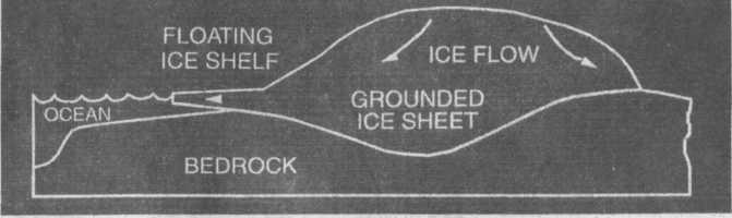
Where ice sheets extend outward to the ocean, the ice tends to move out over the surrounding water, forming “ice shelves.” There is concern that, with global warming, the water under the ice shelves would be warmer and cause them to break up more readily, forming very large icebergs. If the ice shelves of West Antarctica were to break up, this would release more inland ice in an irreversible process, possibly leading to sea level rises of several meters.

SNOW M ИТ

In addition to increasing the amount of melting, global warming would also be expected to increase the amount of precipitation in the polar regions. There are three reasons for this: 1) warmer air can carry more moisture than colder air; 2) warmer wates would encourage increased evaporation from the ocean; and 3) lessened sea ice would also lead to more evaporation from the ocean, as more ocean area would be exposed directly to the atmosphere. Global warming could therefore be expected initially to increase both melting and snowfall. Depending on which increase dominates, the early result could be either an overall decay or an overall growth of the ice sheets.

Global Warming Detection and Sea Ice

The melting and growth of sea ice, in contrast to land ice, does not affect sea level, because the sea ice is floating on the ocean already and is in equilibrium with it. Sea ice is nonetheless still important in the context of climate change. Sea ice, with its high reflectance and the insulation it provides between the polar atmospheres and oceans, is a key part of the climate system. Furthermore, sea ice responds to changes in the atmosphere and oceans, and hence changes in it could be a clue to broader climate change, such as global warming. However, the record to date is not clear enough to make any definitive conclusions about long-term climate trends based on the sea-ice observations alone. Sea ice varies signifi­cantly from season to season and from year to year, and the extent of its natural variability is not yet fully known.

We need to continue to monitor the location and extent of sea ice and its changes seasonally and interannually. We also need additional studies to determine ice thicknesses and reflectivities. This kind of information can be fed into climate models to attempt to simulate future climate conditions. The same information will also serve as a check on models to see if they are properly simulating existing sea-ice amounts and distributions.

NASA Missions to Study Ice

NASA has had missions that collected ice data for many years (see the accompanying table), and ice is among the many variables included in NASA’s Pathfinder Program, which is providing research-quality data sets on global change from past and current satellite missions. The Pathfinder Program will lead up to the main initiative of NASA’s Earth Science Program, the Earth Observing System (EOS). EOS involves a series of satellites to be launched in 1998 and thereafter, providing coverage of the Earth over a period of fifteen to twenty years.

Several sensors on the early satellites in the 1960’s and 1970’s obtained valuable ice data, especially under cloud-free conditions. However, cloudiness and polar darkness often obscured the observations that were obtained with visible and infrared sensors. A major breakthrough occurred in December 1972 with the launch of the Electrically Scanning Microwave Radiometer (ESMR) on the Nimbus-5 satellite. Taking advantage of the microwave radiation that is emitted from the Earth’s surface, ESMR could see through the clouds, providing for the first time detailed data sets of sea-ice distributions for cloudy as well as cloud-free conditions, and could do this at night as well as during daylight.

Microwave radiation is emitted in varying amounts by everything on the surface of the Earth. The amount of radiation emitted depends on the temperature of the substance and its “emissivity,” which is a measure of the substance’s ability to emit radiation. Because the microwave emissivity of sea ice is mark­edly greater than that of water, it generally radiates more microwave energy than the water, even though the temperature of the water is higher. The greater intensity of the microwave radiation coming from ice allows the ice/water distinction to be made in the satellite data.

The data from the Nimbus-5 ESMR and its successor, NASA’s Scanning Multichan­nel Microwave Radi­ometer (SMMR), which was launched on Nimbus-7 in 1978, have resulted in three major atlases, giving the history of the Arctic and Antarctic sea-ice covers for the years 1973-76 and

Antarctic

1978-87. NASA’s Seasat satellite also carried a SMMR instrument in 1978, but, unfortunately, a power failure caused data acquisition to cease after 106 days. The Defense Meteorological Satellite Program (DMSP) has flown a Special Sensor Microwave/Imager (SSM/I) since 1987. This instrument is similar to SMMR, and its data are being analyzed and converted to sea-ice concentrations by NASA and other

scientists.

Seasat also carried a Synthetic Aperture Radar (SAR) able to acquire 25-meter resolution images of the Earth surface in all weather conditions. These data gave NASA scientists the opportunity to demonstrate the powerful capability of SAR for detailed investigations of polar sea ice, and since then, additional SARs have been launched on other satellites.

Data from these recent missions have also enabled scientists to develop new ways to study the vast ice sheets in Greenland and Antarctica. Forinstance, the first high-resolution map (approximately 25 meters) of Antarctica will be compiled from September-October 1997 SAR data obtained by the Cana­dian RADARSAT mission, which was launched in November 1995 by NASA.

Other satellite data also used in the study of ice include data from the Landsat series of satellites and from radar altimetry. For instance, high-resolution Landsat images have been converted into photo maps for parts of the Antarctic and Greenland ice sheets. Landsat images have also been used to measure ice flow rates and the advance and retreat of glacier margins. Radar altimetry data from NASA’s Seasat and the Department of Defense Geosat satellites have been used to determine and map the elevation con­tours of the southern half of the Greenland ice sheet and a small fraction of northern Antarctica. (The Seasat and Geosat orbits did not allow data collection in the central polar regions.)

The EOS series of satellites will carry several important instruments for ice studies starting in 1999. Of particular interest are the Geoscience Laser Altimeter System (GLAS), scheduled to fly in 2001, and the Advanced Microwave Scanning Radiometer (AMSR and AMSR-E), which will fly, respectively, on the ADEOS II mission in 2000 and the EOS PM-1 mission in 2000. AMSR and AMSR-E will obtain sea-ice information with greater spatial detail than earlier microwave radiometers, while GLAS will measure growth or shrinkage of the ice sheets. GLAS will be 100 times more accurate than radar altimeters, which have been designed for ocean measurements, and will be flown in an orbit that reaches very close to flying over the South pole. GLAS measurements of ice melting, changes in snowfall in the polar regions, and changes in ice volume will provide critical data for understanding and predicting sea-level change during the next century. GLAS will also be very useful in the study of individual ice streams and ice shelves in the West Antarctic. Observing these ice streams and shelves is particularly important because of the possibility that they might become unstable under certain conditions of global change.

Sea Ice: Just the Cold Facts

Evaluation: Answers

1. The number of squares will vary depending on the size of the squares on the graph paper. Arctic sea ice is at its maximum in March (end of the Northern Hemisphere winter). Antarctic sea ice is at its maximum in September (end of Southern Hemisphere winter).

2. The Antarctic region has the greatest maximum sea ice coverage (-19 million km² in September), but the Arctic region has the greatest minimum sea ice coverage at approximately 9 million km² in September. Arctic maximum sea ice coverage is approximately 15 million km² in March. Antarctic minimum sea ice coverage is approximately 4 million km² in February. At its maximum, the Arctic is only 79% of the maximum coverage of the Antarctic.

3. The difference between the Arctic and Antarctic sea ice coverage is due to the geography. The area in the central polar region of the Arctic is ocean, bounded largely by the continents of the North­ern Hemisphere. The continental boundaries limit the extent to which Arctic sea ice can grow during the cold months. In contrast, sea ice in the Southern Hemisphere has no land boundaries to the north to limit the winter’s sea ice growth. In the summer, geography again plays a role in sea ice coverage. In the Arctic, the highest-latitude region is covered by water. Arctic sea ice shrinks less in the summer because it lies in an area that stays very cold. The Earth’s south polar region on the other hand, is covered by the'continent of Antarctica. Sea ice extends from the coast of the continent, which is further away from the extreme cold in central Antarctica. The sea ice therefore lies in a relatively warm climate, causing greater melting during the warm summer months.

4. Data are now collected from the Special Sensor Microwave/Imager (SSM/I). Earlier instruments include the Electrically scanning microwave radiometer (ESMR) and the scanning multichannel Mircowave Radiometer (SMMR). An instrument now being built is the Advanced Microwave Scanning Radiometer (AMSR) which is scheduled for flight on the EOS satellites. FYI: Each of these instruments is a passive microwave radiometer, all of which measure microwave radiation given off by objects. Active instruments, like radars, actually send out a signal which they later receive back. Additional information can be found on the ESE CD-ROM in the “How Will We Study the Earth” section.

5. Scientists have measured a global climate change of 0.3 to 0.6 °C over the last 100 years (from the Intergovernmental Panel on Climate Change) and predict further warming in the future. Possible contributions to warming include any reduction in the amount of sea ice coverage and/or any decrease in the amount of time sea ice covers certain areas. Both of these scenarios would lead to a

Sea Ice: Just the Cold Facts

positive feedback. Less sea ice translates into less solar radiation reflected, which would warm the climate and therefore lead to even less sea ice. A greater direct ocean-atmosphere interface uninter­rupted by sea ice would cause an increased heat transfer, especially in the polar winter when the water temperature is often considerably warmer that the air temperature. Conversely, increased sea ice converage would encourage cooling.

The clearing of tropical forests across the Earth has been occuring on a large scale basis for many centu­ries. This process, known as deforestation, involves the cutting down, burning, and damaging of forests.

The loss of tropical rainforest is more profound than merely destruction of beautiful areas. If the current rate of deforestation continues, the world’s rain forests will vanish within 100 years—causing unknown effects on global climate and eliminating the majority of plant and animal species on the planet.

Why Deforestation Happens

Deforestation occurs in many ways. Most of the clearing is done for agricultural purposes—grazing cattle, planting crops. Poor farmers chop down a small area (typically a few acres) and burn the tree trunks—a process called Slash and Burn agriculture. Intensive, or modern, agriculture occurs on a much larger scale, sometimes deforesting several square miles at a time. Large cattle pastures often replace rain forest to grow beef for the world market.

Commercial logging is another common form of deforestation, cutting trees for sale as timber or pulp. Logging can occur selectively-where only the economically valuable species are cut-or by clearcutting, where all the trees are cut. Commercial logging uses heavy machinery, such as bulldozers, road graders, and log skidders, to remove cut trees and build roads, which is just as damaging to a forest overall as the chainsaws are to the individual trees.

The causes of deforestation are very complex. A competitive global economy drives the need for money in economically challenged tropical countries. At the national level, governments sell logging concessions to raise money for projects, to pay international debt, or to develop industry. For example, Brazil had an international debt of $159 billion in 1995, on which it must make payments each year. The logging companies seek to harvest the forest and make profit from the sales of pulp and valuable hardwoods such as mahogany.

Deforestation by a peasant farmer is often done to raise crops for self-subsistence, and is driven by the basic human need for food. Most tropical countries are very poor by U.S. standards, and farming is a basic way of life for a large part of the population. In Brazil, for example, the average annual earnings per person is U.S. $5400, compared to $26,980 per person in the United States (World Bank, 1998). In Bolivia, which holds part of the Amazon rain forest, the average earnings per person is $800. Farmers in these countries do not have the money to buy necessities and must raise crops for food and to sell.

There are other reasons for deforestation, such as to construct towns or dams which flood large areas.

Yet, these latter cases constitute only a very small part of the total deforestation.

The Rate of Deforestation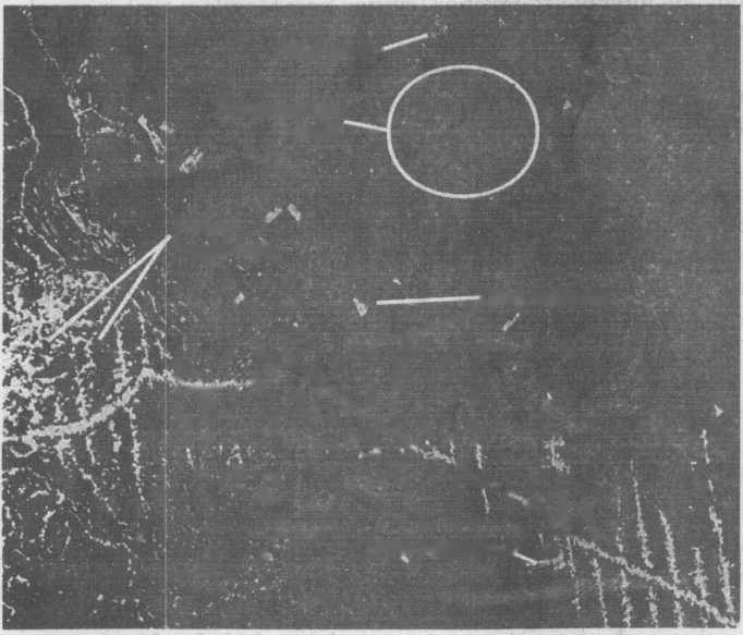

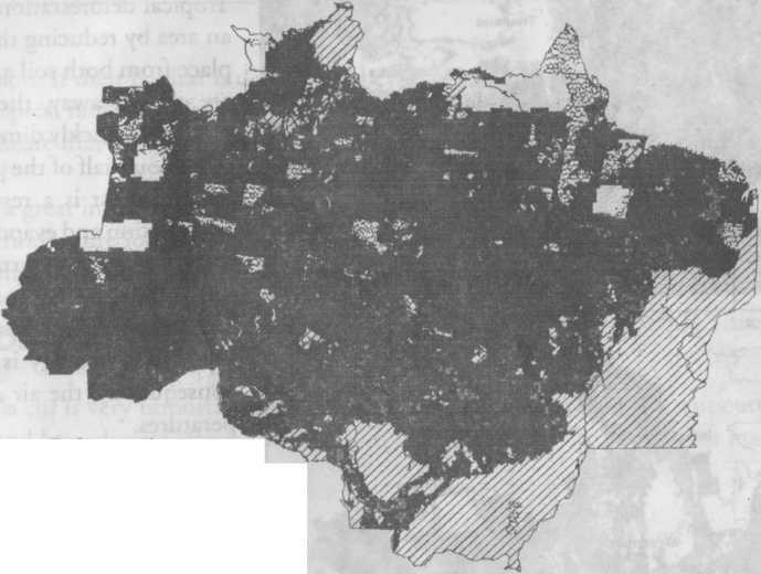
The actual rate of deforestation is difficult to determine. Scientists study the deforestation of tropical forests by analyzing satellite imagery of forested areas that have been cleared. Figure 1 is a satellite image illustrating how scientists classify the landscape. Contained within the image are patches of deforestation in a distinctive “fishbone” of deforestation along roads. Forest fragments are isolated areas left by defores­tation, where the plants and animals are cut off from the larger forest area. Regrowth—also called second­ary forest-is abandoned farmland or timber cuts that are growing back to become forest. The majority of the picture is undisturbed, or “primary,” forest, with a network of rivers draining it.

The Food and Agriculture Organization (FAO) estimates that 53,000 square miles of tropical forests (rain forest and other) were destroyed each year during the 1980s. Of this, they estimate that 21,000 square miles were deforested annually in South America, most of this in the Amazon Basin. Based on these estimates, an area of tropical forest large enough to cover North Carolina is deforested each year!

The rate of deforestation varies from region to region. Recent research results showed that in the Brazil­ian Amazon, the rate of deforestation was around 6200 square miles per year from 1978-1986, but fell to

4800 square miles per year from 1986-1993. By 1988, 6% of the Brazilian Amazon had been cut down (90,000 square miles, an area the size of New England). However, due to the isolation of fragments and the increase in forest/clearing boundaries, a total of 16.5% of the forest (230,000 square miles, an area nearly the size of Texas) was affected by deforestation. Scientists are currently analyzing rates of deforestation for the current decade, as well as studying how deforestation changes from year to year.

У, . jAc; /ГГ/> '

фЩк* A - у

\ Zi ;?■ \ Л \ f44 \ ,

^v Л V: • ili\ i

«"• Deforestations^» ;

■Deforestation

Forest ^J Fragments

Undisturbed

Forest

Regrowth •

The much smaller region of Southeast Asia (Cambodia,

Figure 1. Satellite image of deforestation in the Amazon region, taken from the Brazilian state of Para on July 15, 1986. The dark areas are forest, the white is deforested areas, and the gray is re-growth. The pattern of deforestation spreading along roads is obvious in the lower half of the image. Scattered larger clearings can be seen near the center of the image.

Indonesia, Laos, Malaysia, Myanmar, Thailand, and Vietnam) lost nearly as much forest per year as the Brazilian Amazon from the mid-1970s to the mid-1980s, with 4800 square miles per year converted to agriculture or cut for timber.

Deforestation and the Global Carbon Cycle

Deforestation increases the amount of carbon dioxide (C0₂) and other trace gases in the atmosphere. The plants and soil of tropical forests hold 460-575 billion metric tons of carbon worldwide with each acre of tropical forest storing about 180 metric tons of carbon. When a forest is cut and burned to establish cropland and pastures, the carbon that was stored in the tree trunks (wood is about 50% carbon) joins with oxygen and is released into the at­mosphere as C0₂.

Figure 2, Deforestation in the Brazilian Amazon in 1986. The darker the area, the more forest that is remaining.

Cerrado

Clouds

Deforestation

HI 0-5 percent HI 5 - 20 percent

НИ 20 - 40 percent ЩЦ 40 - 60 percent

HH 60 - 80 percent Я 80 - 100 percent

The loss of forests has a profound effect on the global carbon cycle.

From 1850 to 1990, deforestation worldwide (including the United States) released 122 billion metric tons of carbon into the atmo sphere, with the current rate being approximately 1.6 billion metric tons per year. In

comparison, fossil fuel burning (coal, oil, and gas) releases about 6 billion metric tons per year, so it is clear that deforestation makes a significant contribution to the increasing CO., in the atmosphere. Releasing CO, into the atmosphere enhances the greenhouse effect,-and could contribute to an increase in global

temperatures (see Global Warming Fact Sheet, NF-222).

Figure 3. Deforestation in continental Southeast Asia (excludes Malaysia and Indonesia) from 1973 to 1985. The dark gray represents forest, the lighter areas deforestation. The white box-like areas on the 1985 map are places for which no satellite information was avaliable. During this time period, about 50,000 square miles was deforested.

China and India are included on the map but no assessment of their forest cover was made.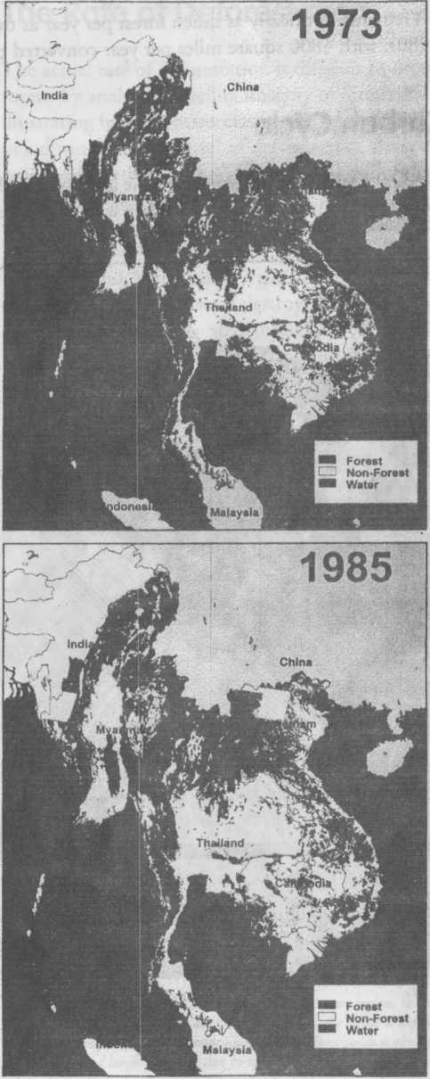

Deforestation and the Hydrologic Cycle

Tropical deforestation also affects the local climate of an area by reducing the evaporative cooling that takes place from both soil and plant life. As trees and plants are cleared away, the moist canopy of the tropical rainforest quickly diminishes. Recent research suggests that about half of the precipitation that falls in a tropi­cal rainforest is a result of its moist, green canopy. Evaporation and evapotranspiration processes from the trees and plants return large quantities of water to the local atmosphere, promoting the formation of clouds and precipitation. Less evaporation means that more of the Sun`s energy is able to warm the surface and, consequently, the air above, leading to a rise in tem­peratures.

Deforestation and Biodiversity

Worldwide, 5 to 80 million species of plants and animals comprise the “biodiversity” of planet Earth. Tropical rain forests—covering only 7% of the total dry surface of the Earth-hold over half of all these species. Of the tens of millions of species believed to be on Earth, scientists have only given names to about 1.5 million of them, and even fewer of the species have been studied in depth.

Many of the rain forest plants and animals can only be found in small areas, because they require a special habitat in which to live. This makes them

Activity	Factors	Time to Regrow
Slash-and-Burn Agriculture	Abandoned rapidly	Less than 50 years
Perennial Shade Agriculture	Some trees left	20 years
Intensive Agriculture	Many pesticides, alteration of hydrology	More than 50 years
Cattle Pasture	Degradation of soils	More than 50 years
Selective Logging	Few trees cut	Less than 50 years
Clearcut Logging	No trees or nutrients left	More than 50 years

very vulnerable to deforestation. If their habitat is destroyed, they may become extinct. Every day, species are disappearing from the tropical rain forests as they are cleared. We do not know the exact rate of extinction, but estimates indicate that up to 137 species disappear worldwide each day.

The loss of species will have a great impact on the planet. We are losing species that might show us how to prevent cancer or help us find a cure for AIDS. Other organisms are losing species they depend upon, and thus face extinction themselves.

After Deforestation

What happens after a forest is cut is very important in the regeneration of that forest. Different cutting techniques and uses of the land have diverse effects on the ground and surviving organisms that make up a rain forest.

In a tropical rain forest, nearly all of the life-sustaining nutrients are found in the plants and trees, not in the ground as in a northern, or temperate forest. When the plants and trees are cut down to sow the land, farmers usually burn the tree trunks to release the nutrients necessary for a fertile soil. When the rains come, they wash away most of the nutrients, leaving the soil much less fertile. In as little as 3 years, the ground is no longer capable of supporting crops.

When the fertility of the ground decreases, farmers seek other areas to clear and plant, abandoning the nutrient-deficient soil. The area previously farmed is left to grow back to a rain forest. However, just as the crops did not grow well because of low nutrients, the forest will grow back just as slow because of poor nutrients. After the land is abandoned, the forest may take up to 50 years to grow back.

Another type of farming practiced in rain forests is called shade agriculture. In this type of farming, many of the original rain forest trees are left to provide shade for shade-loving crops like coffee or choco- late. When the farm is abandoned, the forest grows back very quickly, because much of it was left un­harmed in the first place. After this type of farming, forests can grow back as quickly as 20 years.

Other types of farming can be more devastating for forest regrowth. Intensive agricultural systems use large quantities of chemicals like pesticides and fertilizers. These chemicals kill a lot of the living organ­isms in the area, seeping into the soil and washing into the surrounding areas. On banana plantations, pesticides are used on the plants and in the soil to kill pest animals. However, these pesticides also kill other animals as well, and weaken ecosystem health. Banana plantations also use irrigation ditches and underground pipes for water transport, changing the water balance of the land. After the abandonment of a banana plantation, or other intensive agricultural system, it can take many centuries for a forest to regrow.

A study in Indonesia found that when only 3% of the trees were cut, a logging operation damaged 49% of the trees in the forest. Yet, even with that much damage, the rain forest will grow back relatively quickly if left alone after selective logging, because there are still many trees to provide seeds and protect young trees from too much sun.

Clearcutting is much more damaging to a tropical rain forest. When the land is commercially clearcut and all of the trees removed, the bare ground is left behind with very little regrowth. Unlike when the farmer cleared the land, there are almost no nutrients left behind because all the tree trunks were re­moved. A clearcut forest can require many years to regenerate-in fact, scientists do not know how long it takes for a clearcut forest to grow back.

The Future

The deforestation of tropical rain forests is a threat to life worldwide. Deforestation may have profound effects on global climate and cause the extinction of thousands of species annually. Stopping deforesta­tion in the tropics has become an international movement, seeking ways to stop the loss of rain forests.

Because the loss of rain forests is driven by a complex group of factors, the solutions are equally complex. Simple solutions that do not address the nature of world economics and rain forest ecology have little chance of succeeding. The future requires solutions based on solving the economic crises of countries holding rain forests, as well as improvement of the living conditions of the poor people often responsible for deforestation.

NASA Missions to Study Deforestation

NASA’s Earth Science Enterprise future plans to study the effects of deforestation include continuing analyses using data from such instruments as the Enhanced Thematic Mapper Plus (ETM+), scheduled for flight on Landsat-7, and the Advanced Spaceborne Thermal Emission and Reflection Radiometer (ASTER) and the Moderate Resolution Imaging Spectroradiometer (MODIS), scheduled for flight on the EOS AM-1 satellite. The observational capabilities and scientific studies planned as part of the Earth Science Enterprise, including the Earth Observing System, will help to assess the impacts of deforesta­tion on the global climate system. An overarching objective of the Earth Science Enterprise is to improve our understanding of the causes and effects of climatic and environmental change so that we may be­come more effective and efficient managers of our natural resources, as well as mitigate potential impacts from natural disasters.

существовали в стратосфере, выпущенной из земли и от океанских источников.

Кроме того, ученые находят, что уровни озона периодически изменяются как часть регулярных естественных циклов, таких как изменяющиеся сезоны, ветры, и солнечные циклы. Кроме того вулканические извержения могут ввести материалы в стратосферу, которая может привести к увеличенному разрушению озона.

По Земной целой жизни естественные процессы отрегулировали баланс озона в стратосфере. Простой способ понять баланс озона состоит в том, чтобы думать о прохудившемся ведре. Пока воду льют в ведро при том же самом уровне, что вода просачивается, количество воды в ведре останется тем же самым. Аналогично, пока озон создается при том же самом уровне, что это разрушается, общая сумма озона останется тем же самым.

Начинаясь в начале 1970-ых, однако, ученые нашли доказательства, что деятельность человека разрушает баланс озона. Человеческое производство содержащих хлор химикатов, таких как chlorofluorocarbons (CFCs) добавило дополнительный фактор, который разрушает озон. CFCs - составы, составленные из хлора, фтора и связанного углерода. Поскольку они - чрезвычайно устойчивые молекулы, CFCs действительно бунтуют, реагируют легко с другими химикатами в более низкой атмосфере. Одна из немногих сил, которые могут разбить молекулы CFC, является ультрафиолетовым излучением. В более низкой атмосфере, однако, CFCs защищены от ультрафиолетового излучения озоновым слоем непосредственно. Молекулы CFC таким образом в состоянии мигрировать неповрежденные в стратосферу. Хотя молекулы CFC более тяжелы чем воздух, процессы смешивания атмосферы несут их в стратосферу.

Однажды в стратосфере, молекулы CFC больше не ограждены от ультрафиолетового излучения озоновым слоем. Засыпанный ультрафиолетовой энергией солнца, молекулы CFC разбиваются и выпускают свои атомы хлора. Свободные атомы хлора тогда могут реагировать с молекулами озона, беря один кислородный атом, чтобы сформировать одноокись хлора и оставляя обычную кислородную молекулу.

Если бы каждый атом хлора, выпущенный от молекулы CFC, разрушил только одну молекулу озона, то CFCs представил бы очень немного угрозы озоновому слою. Однако, когда молекула одноокиси хлора сталкивается с freeacorn кислорода, кислородный атом разбивает одноокись хлора, крадя кислородный атом и выпуская атом хлора назад в стратосферу, чтобы разрушить больше озона. Эта реакция происходит много раз, позволяя единственный атом хлора действовать как катализатор, разрушая много молекул озона.

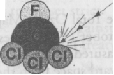
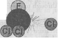
К счастью, атомы хлора не остаются в стратосфере навсегда. Когда свободный атом хлора реагирует с газами, такими как метан (CH4), это перевязано в молекулу водородного хлорида (HC1), который можно нести вниз от стратосферы в тропосферу, где это может быть смыто дождем. Поэтому, если люди прекращают помещать CFCs и другие разрушающие озон химикаты в стратосферу, озоновый слой в конечном счете может восстановить its’elf.

Истощение озона

Термин “озон истощения” означает больше чем только естественное разрушение озона, это означает, что потеря озона превышает создание озона. Думайте снова о “прохудившемся ведре.” Помещение дополнительных разрушающих озон составов, таких как CFCs в атмосферу походит на порождение "ведра" озона к весенним дополнительным утечкам. Дополнительные утечки заставляют озон просачиваться в астре, более быстрой уровнем, чем озон создается. Следовательно, уровень озона, защищающего нас от уменьшений ультрафиолетового излучения.

В области по Антарктиде есть стратосферическое облако, и ледяная беседа частиц не присутствуют в более теплых широтах. Реакции происходят на поверхности ледяных частиц, которые ускоряют разрушение озона, вызванное стратосферическим хлором. Это явление вызвало зарегистрированные уменьшения в концентрациях озона по Антарктиде. Фактически, уровни озона понижаются столь низко весной в южном полушарии, что ученые наблюдали то, что они называют "отверстием" в озоновом слое.

Кроме того, ученые наблюдали уменьшающиеся концентрации озона по целому земному шару. Во второй половине 1993, например, всемирные уровни озона были самыми низкими когда-либо зарегистрированные.

Контроль Озона от Пространства

С 1920-ых озон был измерен от земли. Ученые помещают инструменты в местоположения во всем мире, чтобы измерить количество ультрафиолетового излучения, проходящего через атмосферу на каждом месте. От этих измерений они вычисляют концентрацию озона inthe атмосфера выше того местоположения. Эти данные, хотя полезный в узнавании об озоне, не в состоянии обеспечить соответствующую картину глобальных концентраций озона.

Полный Спектрометр Картографии Озона (TOMS), который инструмент, которым сначала управляют на Нимбе 7 спутников в октябре 1978, ежедневно делает, международные наблюдения за общей суммой озона в атмосфере, измеренной в масштабе Добсона (см. следующий параграф). TOMS измеряет солнечный свет, который был рассеян назад к пространству от атмосферы в многократных длинах волны. Так как озон поглощает ультрафиолетовый свет, чем больше существующего озона, тем менее отраженное ультрафиолетовое излучение. Чтобы иллюстрировать этот принцип, предположите лить немного воды в мензурку и измерять количество. Повторите процедуру, но теперь поместите губку между стаканом и мензуркой. Начиная с действий озона как губка, поглощая УЛЬТРАФИОЛЕТОВУЮ радиацию, меньше проходит на поверхность Земли, и также меньше отражено, отступают, чтобы сделать интервалы.

Некая единица Добсона обращается к слою озона, который был бы 0.001 см толщиной при условиях стандартной температуры (0°C) и стандартного давления (1013.25 millibars, среднее давление в поверхности Земли). Таким образом, например, 300 единиц Добсона озона, сниженного на поверхность Земли в 0°C, заняли бы слой только 0.3 см толщиной! Когда единицы Добсона падают ниже 225, отверстие, как говорят, существует (так как есть фактически все еще некоторый озон в стратосфере, это не отверстие в традиционном смысле, но количество не достаточно препятствовать тому, чтобы значительное вредное ультрафиолетовое излучение достигло поверхности Земли). С меньшим количеством озона, чтобы поглотить вредные ультрафиолетовые лучи, больше ультрафиолетового излучения получено в поверхности нашей планеты. Количество озона может быть сравнено от области до области по обширным областям цветом, кодирующим единицы измерения от масштаба Добсона.

Вопреки изображению, созданному термином “, озонового слоя” количество и распределение молекул Озона в стратосфере изменяется очень по земному шару. Молекулы озона транспортируются вокруг стратосферы очень, как водные облака транспортируются в тропосфере. Поэтому, ученые, наблюдающие колебания озона только, одно пятно не могло знать, означало ли изменение в местных уровнях озона изменение в глобальных уровнях озона, или просто колебание в концентрации по тому особому пятну. Спутники дали ученым способность преодолеть эту проблему, потому что они обеспечивают картину того, что происходит одновременно по всей Земле.

Продолжающаяся контрольная программа озона в стадии реализации использует TOMS. Инструментами TOMS управляли на российском Метеоре 3 полярно орбитальных спутника в 1991 и на японском Продвинутом Земном Спутнике Наблюдения 1 (ADEOS-1) в 1996. Дополнительные инструменты TOMS, как намечают, будут управлять на нескольких системах наблюдения Земли (ЭОС) спутниками в будущем.

Ученые теперь уверены, что стратосферический озон исчерпывается во всем мире частично из-за деятельности человека. Однако, ученые все еще не знают, сколько из потери результат деятельности человека, и сколько результат колебаний innatural циклы.

Предсказание Уровней Озона

Если ученые могут отделить человеческие и естественные причины истощения озона, они могут сформулировать улучшенные модели для того, чтобы предсказать уровни озона. Предсказания ранних моделей уже использовались политикой

производители, чтобы определить, что могут быть сделаны, чтобы уменьшить истощение озона, вызванное людьми. Например, сталкивающийся с большой вероятностью, что CFCs мог нанести серьезный ущерб озоновому слою, тактики со всего мира в 1987 подписали соглашение, известное как Монреальский Протокол. Это соглашение устанавливало строгие пределы для производства и использования CFCs. К 1990 растущее количество научного доказательства против CFCs побудило дипломатов усиливать требования Монреальского Протокола. Пересмотренное соглашение призывало к полному постепенному сокращению производства CFC в развитых странах к 1996 году.

Однако, ученые соглашаются так, что много остается быть изученным о взаимодействиях тот озон аффекта. Чтобы создать точные модели, ученые должны изучить одновременно все факторы, затрагивающие создание озона и разрушение. Кроме того они должны изучить эти факторы от пространства непрерывно за многие годы, и по всему земному шару. Система наблюдения Земли НАСА (ЭОС) позволит ученым изучать озон только этим способом. Серия ЭОС спутников будет нести искушенную группу инструментов, которые измерят взаимодействия в пределах атмосферы тот озон аффекта. Основываясь на многих годах данных, собранных предыдущими миссиями НАСА, эти измерения увеличат резко наше знание химии и динамику верхней атмосферы и наше понимание того, как деятельность человека затрагивает защитный озоновый слой Земли.

Сезонные Изменения Озона

Стратосферические уровни озона изменяются быть сезоном и широтой. С 1979 середина широты (30 ° - 60 °) уровни озона упала приблизительно на 5 %. Создание озоновой дыры вовлекает высокие концентрации хлора, полярных стратосферических облаков, и вихря сильного ветра (названный полярным вихрем). Потеря озона ускорена по Антарктиде, потому что стратосфера содержит ледяные частицы, которые мешают хлору и брому быть включенными в “безопасные молекулярные формы” и увеличивать их роль разрушительных химикатов, которые могут сломать обособленно молекулы озона с удивительной эффективностью. В течение полярной ночи, когда несколько месяцев темноты спускаются на Антарктиде, грузиле температур ниже-80°C. Реальное действие начинается, когда Солнце возвращается к этой части мира во время весенней поры, возбуждая химический цикл, который разрушает озон.

Воздействия на здоровье Ультрафиолетового излучения

Мы также измеряем количество ультрафиолетового излучения, достигающего поверхности. Ультрафиолетовый свет, ОСОБЕННО УЛЬТРАФИОЛЕТОВЫЙ-B, может быть опасным. Это может вызвать непосредственные эффекты, такие как горячие загары, так же как более долгий срок - проблемы как рак кожи и катаракты. Более высокие уровни могут подавить иммунную систему, и понизить население фитопланктона (фитопланктон включают основание морской пищевой сети). Для каждого 1%-ого уменьшения в стратосферическом озоне там вычислен, чтобы быть 2%-ым увеличением количества солнечного ультрафиолетового излучения, достигающего земли. Это могло увеличить число случаев рака кожи на 3 % к 6 % ежегодно.

В 1994 Национальная метеорологическая служба и Управление по охране окружающей среды развивали Ультрафиолетовый (УЛЬТРАФИОЛЕТОВЫЙ) Индекс как способ определить количество количества подвергания ультрафиолетовому излучению в течение определенного дня. Индексы колеблются от 0 до 10 +. В соединении с УЛЬТРАФИОЛЕТОВЫМ Индексом EPA начало бесплатную Стратосферическую информацию об Озоне Горячая линия (1-800-296-1996). Гости могут просить информацию о том, как Соединенные Штаты осуществляют стратосферическую политику озона.

Облака и энергетический Цикл

Исследование облаков, где они происходят, и их особенности, может хорошо быть центральным ключом к пониманию изменения климата. Низко, густые облака прежде всего отражают солнечное излучение и охлаждают поверхность Земли. Высокие, тонкие облака прежде всего передают поступающее солнечное излучение; в то же самое время они заманивают часть в ловушку коммуникабельной инфракрасной радиации, испускаемой Землей, и излучают это назад вниз, таким образом нагревая поверхность Земли.

Нагреется ли данное облако или охладится, поверхность зависит от нескольких факторов, включая высоту облака, ее размер, и состав частиц, которые формируют облако. Баланс между охлаждением и нагреванием действий облаков очень близок, хотя, в целом, составляя в среднем эффекты всех облаков во всем мире, охлаждение преобладает.

Система климата Земли постоянно приспосабливается в пути, который склоняется к поддержанию баланса между энергией, которая достигает Земли от солнца и энергии, которая идет от Земли, отступают, чтобы сделать интервалы. Ученые именуют это как “радиационный бюджет Земли.” Компоненты Земной системы, которые важны для радиационного бюджета, являются поверхностью планеты, атмосферой, и облаками. Энергию, прибывающую от солнца до поверхности Земли, называют солнечной энергией. Большая часть из этого находится в форме радиации от "видимых" длин волны, то есть, ответственные за свет, обнаруженный нашими глазами. Видимая радиация и радиация с более короткими длинами волны, такими как ультрафиолетовое излучение маркированы "короткая волна". И количеством энергии и длинами волны, в которых энергия испускается любой системой, управляет средняя температура поверхностей излучения системы плюс свойства эмиссии. Температура поверхности излучения солнца, или фотосфера, является больше чем 5500°C (9900°F). Однако, не вся энергия солнца прибывает в Землю. Энергия солнца испускается во всех направлениях с только небольшой частью, являющейся в направлении Земли.

Энергия возвращается, чтобы сделать интервалы от Земной системы двумя способами: отражение и эмиссия. Часть солнечной энергии, которая прибывает в Землю, отражена, отступают, чтобы сделать интервалы в том же самом, коротких длинах волны, в которых это прибыло в Землю. Фракцию солнечной энергии, которая отражена назад, чтобы сделать интервалы, называют альбедо. У различных частей Земли есть различные альбедо. Например, у океанских поверхностей и дождевых лесов есть низкие альбедо, что означает, что они отражают только небольшую часть энергии солнца. У пустынь, льда, и облаков, однако, есть высокие альбедо; они отражают значительную часть энергии солнца. По целой поверхности Земли приблизительно 30 процентов поступающей солнечной энергии отражены назад, чтобы сделать интервалы. Поскольку у облака обычно есть более высокое альбедо чем поверхность ниже этого, облако отражает больше коротковолновой радиации назад, чтобы сделать интервалы, чем поверхность была бы в отсутствие облака, таким образом оставляя меньше солнечной энергии, доступной, чтобы нагреть поверхность и атмосферу. Следовательно, это “принуждение альбедо облака,” взятый отдельно, имеет тенденцию вызывать охлаждение или “отрицательное принуждение” климата Земли. Коротковолновое отражение облаками иллюстрировано в рисунке 1.

Другая часть энергии, собирающейся сделать интервалы от Земли, является электромагнитной радиацией, испускаемой Землей. Солнечное излучение, поглощенное Землей, заставляет планету нагреваться вплоть до этого, испускает так много энергии назад в космос, как это поглощает от солнца. Поскольку Земля поглощает только крошечную фракцию энергии солнца, это остается более прохладным чем солнце, и поэтому испускает намного меньше радиации.

Большая часть этой радиации в более длинных длинах волны чем солнечное излучение. В отличие от солнечного излучения, которое является

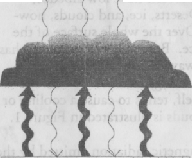
противостоящее альбедо облака и оранжерея облака forcings определяют, добавит ли определенный тип облака к естественному нагреванию воздуха поверхности Земли или окажет охлаждающееся влияние. Как объяснено ниже, высокие тонкие облака усика имеют тенденцию увеличивать нагревающийся эффект, и низко у толстых stratocumulus облаков есть противоположный эффект, в то время как глубоко конвективные облака нейтральны. Полный эффект всех облаков вместе состоит в том, что поверхность Земли более прохладна, чем это было бы, если бы у атмосферы не было никаких облаков.

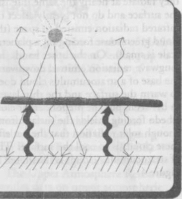
Высокие Облака

Высокие, тонкие облака усика в атмосфере Земли действуют в пути, подобном прозрачному воздуху, потому что они очень прозрачны к коротковолновой радиации (их принуждение альбедо облака является маленьким), но они с готовностью поглощают коммуникабельную longwave радиацию. Как прозрачный воздух, облака усика поглощают радиацию Земли и затем испускают longwave, инфракрасная радиация и чтобы сделать интервалы и отступить на поверхность Земли. Поскольку облака усика являются высокими, и поэтому холодными, энергия, излученная к космосу, ниже, чем это было бы без облака (принуждение оранжереи облака является большим). Часть радиации, таким образом пойманной в ловушку и отосланной назад к поверхности Земли, добавляет к коротковолновой энергии от солнца и longwave энергии от воздуха, уже достигающего поверхности. Дополнительная энергия вызывает нагревание поверхности и атмосферы. Полный эффект высоких тонких облаков усика тогда состоит в том, чтобы увеличить атмосферное нагревание оранжереи. Эффект облаков усика иллюстрирован в рисунке 3.

Низкие Облака

В отличие от эффекта нагревания более высоких облаков, низко stratocumulus облака действуют, чтобы охладить Земную систему. Поскольку более низкие облака являются намного более толстыми чем высокие облака усика, они не столь прозрачны: они не позволяют такой большой солнечной энергии достигать поверхности Земли. Вместо этого они отражают большую часть солнечной энергии назад, чтобы сделать интервалы (их принуждение альбедо облака является большим). Хотя stratocumulus облака также испускают longwave радиацию, чтобы сделать интервалы и к поверхности Земли, они около поверхности и при почти той же самой температуре как поверхность. Таким образом, Облака

они исходят в почти той же самой интенсивности как поверхность и не очень затрагивают инфракрасную радиацию, испускаемую, чтобы сделать интервалы (их принуждение оранжереи облака в планетарном масштабе является маленьким). С другой стороны longwave радиация, испускаемая вниз от основы stratocumulus облака, действительно имеет тенденцию нагревать поверхность и тонкий слой воздуха промежуточный, но преобладающее принуждение альбедо облака ограждает поверхность от достаточного количества солнечного излучения, что результирующий эффект этих облаков состоит в том, чтобы охладить поверхность. Эффект stratocumulus облаков иллюстрирован в рисунке 4.

Глубоко Конвективные Облака

В отличие от обеих из категорий облака, ранее обсужденных, глубоко конвективные облака, символизированные cumulonimbus облаками. cumulonimbus облако может быть много километров толщиной с основой около поверхности Земли и вершины, часто достигающей высоты 10 км (33 000 футов), и иногда намного выше. Поскольку cumulonimbus вершины облака являются высокими и холодными, энергия, излученная к космосу, ниже, чем это было бы без облака (принуждение оранжереи облака является большим). Но потому что они также являются очень толстыми, они отражают большую часть солнечной энергии назад, чтобы сделать интервалы (их принуждение альбедо облака является также большим); следовательно, с уменьшенной коротковолновой радиацией, которая будет поглощена, нет по существу никакой лишней радиации, которая будет поймана в ловушку. Как следствие, в целом, оранжерея облака и альбедо forcings почти балансируют, и полный эффект cumulonimbus облаков нейтрален - ни нагревание, ни охлаждение. Эффект глубоких конвективных облаков иллюстрирован в рисунке 5.

Переменная Ключа облаков-A в Глобальном Изменении

Эффект облаков на климате зависит от соревнования между отражением поступающего солнечного излучения и поглощением коммуникабельной инфракрасной радиации Земли.

Низкие облака имеют охлаждающийся эффект, потому что они являются оптически толстыми и отражают большую часть поступающего солнечного излучения, чтобы сделать интервалы.

Высокие тонкие облака усика имеют эффект нагревания, потому что они передают большую часть поступающего солнечного излучения, в то время как в то же самое время они заманивают часть в ловушку инфракрасной радиации Земли и излучают ее назад на поверхность.

Глубоко конвективные облака, в среднем не имейте ни нагревания, ни охлаждающегося эффекта, потому что их оранжерея облака и альбедо forcings, хотя оба большие, почти отмените друг друга.

Миссии НАСА Изучить Облака и энергетический Цикл

Исследования облаков и энергетического цикла были выполнены много лет как часть многих миссий НАСА. В ближайшем будущем маленькие миссии, обращаясь к определенным исследованиям запланированы, приводящий к главной инициативе Программы Науки о Земле НАСА, система наблюдения Земли (ЭОС) серия спутников, начинающихся в 1999.

Исторически, Телевизионный Инфракрасный Спутник Наблюдения (НОВИЧКИ) ряд обеспечил технологический тест, чтобы получить ежедневные температурные и глобальные данные облачного покрова. Ряд Нимба обеспечил первый глобальный радиационный анализ бюджета от пространства, указывая, что планетарное альбедо было ниже и коммуникабельная инфракрасная радиация выше чем ранее веривший. Земной Радиационный Эксперимент Бюджета (ERBE) обеспечил улучшенный и более - всесторонний анализ глобального радиационного бюджета и, особенно, первых глобальных наблюдений за оранжереей облака и альбедо forcings. Верхний Исследовательский спутник Атмосферы (UARS) контролирует солнечную энергию, достигающую Земли, и обеспечивает данные по верхней атмосферной химии и динамике. Ранний Спейслэб/Космическая транспортная система (STS) и Атмосферная Лаборатория для Заявлений и Науки (АТЛАС) полезные грузы, начатые на Шаттле, обеспечили данные по солнечной энергии, взаимодействиям атмосферы солнца, и верхней атмосферной химии и динамике.

Следующие Шаги

Важная миссия для исследования облаков - объединенные США/Япония Тропическая Миссия Измерения Ливня (TRMM). TRMM, начатый в ноябре 1997, несет Облака ЭОС и Сияющую энергетическую систему Земли (ВОСКОВИНЫ) инструмент, улучшенная версия инструментовки ERBE. Кроме того, TRMM несет инструментовку, чтобы изучить испарение водного пара в атмосферу и ее уплотнение, чтобы произвести ливень, процессы основной важности для глобального энергетического бюджета. Несколько из серий ЭОС спутников будут нести инструмент ВОСКОВИН и другую продвинутую инструментовку, чтобы обеспечить чрезвычайно - точный, последовательный, и долгосрочный (15 лет) радиационная база данных и облако. Исследования этих данных, основываясь на начале, положенном предыдущими миссиями, приведут к лучшему пониманию роли облаков и энергетического цикла в глобальном изменении климата. Вулканы

Вулканы и Глобальное Охлаждение

Вулканические газы, как думают, ответственны за глобальное охлаждение, которое иногда наблюдалось в течение нескольких лет после главного извержения. Недавние исследования показали, что, когда аэрозоли сульфата, выпущенные вулканическими извержениями, достигают стратосферы, они могут оказать большое, широко распространенное влияние охлаждения. Аэрозоли отражают, что много поступающего солнечного излучения отступает, чтобы сделать интервалы и поэтому создать чистый эффект охлаждения на поверхность Земли. Фактически 1992, после извержения Mt. Pinatubo в июне 1991, был один из самых прохладных лет на отчете.

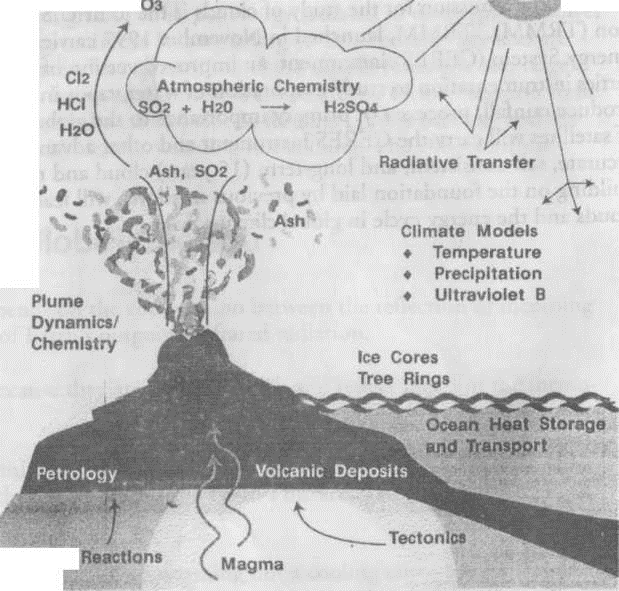
Рассеивание аэрозолей зависит от изгнанного количества, угол и сила изгнания, и широта возникновения. Если вулкан изгонит материал из своей стороны, то большая часть двуокиси серы останется в тропосфере и не будет широко рассеяна. Однако, если материал изгнан вертикально и входит в стратосферу, есть увеличенные возможности, что аэрозоли будут широко распределены преобладающими поясами ветра нашей планеты. Меньше смешивания происходит между высокими latitiude поясами ветра и остальной частью планеты, особенно в течение полярных зим, и поэтому, вулканы, которые прорываются в высоких широтах (60 ° +), менее вероятно, будут иметь глобальные эффекты. Противоположность верна для середины. '"и низкие извержения широты, потому что есть большое количество W смешивания между ними.

Mt. Pinatubo, прорвался 15 июня 1991.

Расположенный на Филиппинах в 15.0 °N и 120.0°E, облако аэрозоля поехало на запад с преобладающими ветрами.

Больше чем 5 миллиардов кубических метров пепла и пирокластических развалин были изгнаны из вулкана. Извержение вызвало 847 смертельных случаев, 184 раны, и переместило приблизительно 1 миллион человек.

Рисунок 1 иллюстрирует, что, поскольку вулканы прорываются, они взрывают огромные облака в атмосферу. Эти облака составлены из частиц и газов, включая двуокись серы. Миллионы тонн газа двуокиси серы могут достигнуть стратосферы от главного извержения.

Там, двуокись серы преобразовывает в крошечную постоянную серную кислоту

(сульфат) частицы, упомянутые asaerosols. Эти sulfare частицы отражают энергию, прибывающую из солнца, таким образом уменьшая количество достижения солнечного света и нагревания поверхности Земли.

Краткосрочное глобальное охлаждение часто связывалось с некоторыми главными вулканическими извержениями. 1816 год упоминался как “год без лета.” Это было время существенного связанного с погодой разрушения в Новой Англии и в Западной Европе с убийством летних морозов в Соединенных Штатах и Канаде. Эти странные явления были приписаны главному извержению вулкана Tambora в 1815 в Индонезии. Вулкан бросил газ двуокиси серы в стратосферу, и слой аэрозоля, который сформировался, привел к блестящим закатам, замеченным во всем мире в течение нескольких лет.

Но, не все вулканические извержения, не даже все большие вулканические извержения, производят охлаждение глобального масштаба.

Гора Аганг в 1963 очевидно вызвала значительное уменьшение в температурах вокруг большой части мира, тогда как эль Chichon в 1982, казалось, имел небольшой эффект, возможно из-за его различного местоположения или из-за Эль-Ниньо, который произошел тот же самый год. (См. главу Эль-Ниньо.) Эль-Ниньо - явление Тихого океана, но он вызывает международные погодные изменения, которые, возможно, действовали, чтобы уравновесить эффект эль извержения Chichon.

Вулканы и Истощение Озона

Другой возможный эффект вулканического извержения - разрушение стратосферического озона. Исследователи теперь предполагают, что частицы аэрозоля, содержащие серную кислоту от вулканической эмиссии, могут способствовать потере озона. Когда составы хлора, следующие из распада chlorofluorocarbons (CFCs) в стратосфере, присутствуют, частицы сульфата могут служить, чтобы преобразовать их в более - активные формы, которые могут вызвать более - быстрое истощение озона. (См. главу Озона.)

Контроль Эффектов Вулканов

Основанные на пространстве инструменты - единственный практический способ наблюдать большие и преходящие вулканические облака извержения. Полный Спектрометр Картографии Озона НАСА (TOMS) инструменты способствовал значительно нашему знанию общей суммы двуокиси серы, испускаемой в атмосферу в ходе главных вулканических извержений. Рисунок 2 показывает изображения TOMS двуокиси серы, распространяющейся через Район Индийского океана после извержения Горы Пинэтубо. Несколько недель спустя двуокись серы распространила во всем мире как наблюдающийся Микроволновым Эхолотом Конечности (МЛ) инструмент на Верхнем Исследовательском спутнике Атмосферы НАСА (UARS) (рисунок 3).

В дополнение к обнаружению двуокиси серы из Горы Пинэтубо TOMS сделал подобные наблюдения больше чем за 100 вулканическими событиями, включая главное извержение от Гудзонского вулкана Cerro в Чили в 1991. Инструменты TOMS были начаты на Нимбе 7 космических кораблей в 1978; российский Метеор 3 космических корабля в 1991; и на Земном Исследовании и японской Продвинутой системе наблюдения Земли (ADEOS) платформы в 1996. Инструмент АТОМОВ, как также намечают, полетит на российском-3M спутнике в 2000.

Данные от Стратосферического Аэрозоля и Газового Эксперимента (МУДРЕЦ II) инструмент на Земном Радиационном Спутнике Бюджета НАСА (ERBS) показали это в течение первых пяти месяцев после Горы

О

Ми Pinatubo 18 ИЮНЯ. 19У1

Рисунок 2: Изображения от Нимба-7 TOMS показ распространения двуокиси серы от Mt. Извержение Pinatubo. "Шкала яркости" указывает, что толщина слоя двуокиси серы имела бы если наблюдающийся при стандартных поверхностных условиях температуры и давления.

Извержение Pinatubo, оптическая глубина стратосферического аэрозоля увеличилась до 100 раз в определенных местоположениях. Оптическая глубина - общая мера способности области атмосферы, чтобы предотвратить проход видимого света через это. Большие оптические глубины означают большую блокировку света. В этом случае увеличенная оптическая глубина означает, что значительно меньше энергии солнца может пройти через облако, чтобы нагреть поверхность Земли. Продвинутый МУДРЕЦ III инструментов, которые сделают подобные наблюдения, как намечают, будет начат на российском Метеоре - 3M космический корабль во второй половине 1998.

Наблюдения за эффектами Mt. Аэрозоли Pinatubo на мировом климате использовались, чтобы утвердить понимание ученых изменения климата и нашей способности предсказать будущий климат. Исследователи в Институте космических исследований имени Годдарда НАСА в Нью-Йорке применили свою модель общей циркуляции климата Земли к проблеме. Они сообщили об успехе в правильном предсказании многих из эффектов аэрозолей сульфата от извержения Пинэтубо Горы при понижении глобальных температур.

Миссии НАСА Изучить Вулканы

Некоторые из прошлых и настоящих миссий НАСА, которые способствуют исследованию вулканов, перечислены в сопровождающем столе. Включенный в стол система наблюдения Земли (ЭОС), основной элемент Earth Science Enterprise НАСА. Первый запуск в серии спутников ЭОС, как намечают, будет иметь место в 1998.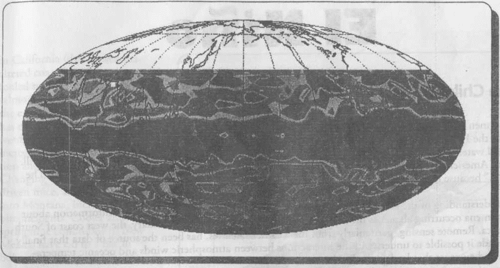

Рисунок 3. Изображения от облака спутниковой двуокиси серы UARS от Mt. Pinatubo 23 сентября 1991, после рассеивания во всем мире

Высокое разрешение Инфракрасный Радиометр (HRIR), которым сначала управляют на Нимбе НАСА 1 спутник в 1964, использовалось, чтобы наблюдать и активные и бездействующие вулканы. На Нимбе 2, HRIR сделал запись энергетических изменений от вулканической деятельности по Surtsey, Исландия в 1966. Многоспектральный Сканер (Г-ЖА) и Тематический Картопостроитель (ТМ) инструменты на спутниках Landsat обеспечил длинную серию изображений вулканической деятельности, таких как выражение, вулканические падения пепла, и потоки лавы.

Программа EOS включит серию спутников, которые будут нести продвинутые инструменты, чтобы обеспечить чрезвычайно точную, последовательную, и долгосрочную базу данных многих аспектов Земной атмосферы, земли, и океанских особенностей. Информация, полученная от этого серьезного усилия, чтобы изучить Земные явления, расширит наше знание взаимодействий вулканов с климатом Земли.

Глоссарий Химии

Статья,

молекула хлора

HC1

водородный хлорид

н, о

вода

°3

озон

серная кислота

ТАК,

двуокись серы

Ребенок

Рыбаки, которые сгибают воды Тихого океана недалеко от берега Перу и Эквадора, знали в течение многих столетий об Эль-Ниньо. Каждые три - пять лет в течение месяцев декабря и января, рыбы в прибрежных водах прочь этих стран фактически исчезают, заставляя рыбацкий бизнес зайти в тупик. Южноамериканские рыбаки дали этому явлению имя Эль-Ниньо, который является испанским для “Ребенка,”, потому что это появляется время празднования рождения Младенца Христа.

Понимание сложных процессов на работе, чтобы произвести Эль-Ниньо запрашивает информацию о явлениях, происходящих все через тропический Тихий океан: не только его восточная граница, западное побережье Южной Америки. Дистанционное зондирование, особенно от метеорологических спутников, было источником данных, которые наконец позволили понять взаимодействия между атмосферными ветрами и океанскими температурами и потоками, которые приводят к Эль-Ниньо.

Международные Эффекты

Ближе к домашнему Эль-Ниньо годы были связаны с изменением Северных Тихоокеанских атмосферных и океанских потоков, приносящих более теплые воды к западному побережью Вашингтона, Орегона, и Callifornia. Эти изменения были ответственны за увеличенные нападения акулы от Орегонского побережья, увеличились, спинная injuriesin Калифорния (из-за погоды - изменил прибрежные морские этажи, которые дурачили серфингистов), и изменения в популяциях лососей. Кроме того, восточное побережье Соединенных Штатов испытало более теплые и более влажные условия весенней поры, увеличивая популяцию москитов и случаи энцефалита. Изменяющиеся метеорологические карты гнали мышей, и поэтому змей в Монтану, увеличивая инциденты укуса змеи. Более прохладные и более влажные условия весенней поры в Нью-Мексико привели к повышению бубонной чумы, поскольку популяция грызунов увеличилась.

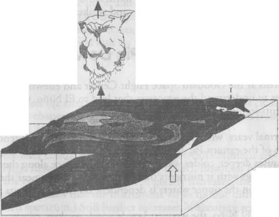
Взаимодействие воздуха/Моря

Основной элемент явления Эль-Ниньо - взаимодействие между ветрами в атмосфере и морской поверхности. Без этого взаимодействия воздуха/моря не было бы никакого Эль-Ниньо. Используя в своих интересах наблюдения от Национального управления океанических и атмосферных исследований (NOAA) метеорологические спутники, ученые были в состоянии отследить движущиеся образцы морских температур поверхности. Бассейн с теплыми водами, который обычно проживает в западных водах Тихого океана, как замечалось, дрейфовал в восточном направлении к западному побережью Южной Америки.

T его предсказывает появление Эль-Ниньо.

Изображения спутника НАСА также помогают нам видеть движущиеся образцы штормов по экватору, которые являются последствием движущихся местоположений ofthe бассейн теплой воды. Высокие облака кучи, достигая высоко в атмосферу с многократными областями сильных - и - вниз вертикальные (конвективные) движения, форма и движение в восточном направлении через Тихий океан, поскольку они произведены теплыми поверхностными водами. Это движение сильно активных конвективных областей изменяет поверхностные ветры, и ослабляет обычно преобладающий восток на запад торговые ветры. (См. рисунки 1 и 2.)

Космические Наблюдения Придавливают Явление Эль-Ниньо

Ученые из Центра космических полетов имени Годдарда и в другом месте использовали числовые модели и теоретические исследования, чтобы понять процессы, которые приводят к Эль-Ниньо. Сравнение с данными показало последовательность событий, приводящих к Эль-Ниньо.

В нормальных годах, когда нет никакого Эль-Ниньо, торговые ветры имеют тенденцию дуть с востока на запад через воды восточного Тихого океана. Они имеют тенденцию тянуть поверхностные воды на запад через океан. В свою очередь это заставляет глубже, более холодные воды повышаться до поверхности вдоль побережья. "Резко поднимание" глубоких океанских вод приносит с этим питательные вещества, которые иначе легли бы около дна океана. Популяция рыб, живущая в верхних водах, зависит от этих питательных веществ снизу для выживания.

Во время Эль-Ниньо движущиеся на запад торговые ветры слабеют, вызывая резко поднимание глубоководных прекратиться. Последовательное нагревание океанской поверхности далее ослабляет торговые ветры, и усиливает Эль-Ниньо. Без резко поднимания питательные вещества от глубоководного больше не доступны. Это сигнализирует серьезное сокращение рыбной промышленности до времени, когда нормальные условия возвращаются.

Предсказание событий Эль-Ниньо - теперь центр главной научной инициативы. Предсказание Эль-Ниньо требует, чтобы сложные числовые модели моделировали: 1) изменения в пределах океана та поверхность причины

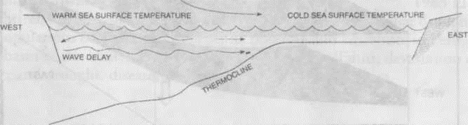
Схематичный из главных процессов, которые, как думают, произвели Эль-Ниньо. Выше-нормального морские температуры поверхности производят увеличенное осаждение и изменения в атмосферном обращении. Они имеют тенденцию поддерживать теплые температуры, ведя океанские потоки. Некоторые из этих эффектов являются немедленными; другие действуют после того, как принудительный сигнал размышляет от западной границы и возвращается в область сильного cou-pling.

.temperatures к теплому; 2) изменения в атмосферной конвекции и облаках, должных появляться, нагревая; и 3) изменения в поверхностных ветрах, которые вызваны конвективными беспорядками. Социальные воздействия точного прогноза Эль-Ниньо до года заранее огромны, позволяя экономическую политику и производителей аграрной политики приспособиться к краткосрочным колебаниям климата выгодным способом. Спутниковые наблюдения продолжат играть важную роль в обеспечении успеха этих прогнозов, обеспечивая точные измерения существующих условий в регионе, существенной первой задаче для предсказания.

Миссии НАСА Изучить Эль-Ниньо

За эти годы несколько миссий НАСА изучили эффекты, связанные с Эль-Ниньо, такие как изменения в поверхностной морем температуре изменения облачного покрова и (SST). Эти исследования увеличены данными от эксплуатационных спутников Национального управления океанических и атмосферных исследований (NOAA).

Начальные усилия при картографии SST и облачного покрова проводились, используя данные от серии Нимба НАСА спутников. Продвинутый Радиометр Очень С высоким разрешением с четырьмя каналами (AVHRR), которым управляют на метеорологическом спутнике НОВИЧКОВ-N NOAA в 1978 и на спутнике NOAA-6 в 1979, очень увеличил точные измерения эффектов Эль-Ниньо. (“Четыре канала” означают, что инструмент рассматривает в четырех различных частях электромагнитного видимого и инфракрасного спектра.) Все еще дальнейшие увеличения точности закончились, когда пятый канал был добавлен к инструменту AVHRR, которым управляют на NOAA-7 в 1981, и на последующих спутниках NOAA. Пятый канал улучшил измерение SST, обеспечивая исправления для атмосферного водного пара, который иначе вмешается в температурные измерения.

Объединенная американско-французская миссия TOPEX/Poseidon была начата в 1992 и обеспечивает глобальные определения изменений в океанских поверхностных потоках, которые связаны с явлением Эль-Ниньо. Потоки определены от изменений в океанских поверхностных возвышениях, измеренных высотомерами на TOPEX/Poseidon с точностью нескольких сантиметров.

НАСА начало “Программу Первооткрывателя”, чтобы сделать доступные данные более высокого качества из прошлых и текущих миссий. Эти усилия приведут к системе наблюдения Земли (ЭОС), главная инициатива Earth Science Enterprise НАСА. В 1998 будет начато первое в серии спутников ЭОС.

Объединенная американско-японская Тропическая Миссия Измерения Ливня (TRMM), начатый 27 ноября 1997, использует впервые, и активный (радар) и пассивные микроволновые датчики от пространства, чтобы обеспечить измерения осаждения, облаков, и радиационных процессов в более низких широтах, включая части Тихого океана, где Эль-Ниньо происходит.

НАСА scatterometer названный NSCAT управляло на японской Продвинутой системе наблюдения Земли (ADEOS) космическим кораблем, который был запущен в августе 1996. NSCAT обеспечил очень высококачественные данные по скорости и руководству океански-поверхностных ветров во всем мире. К сожалению, после девяти месяцев в орбите, относящийся к космическому кораблю отказ закончил поток чрезвычайно ценных данных NSCAT. Признавая существенные вклады в Науку о Земле, сделанную NSCAT, НАСА теперь планирует начать копию нового SeaWinds scatterometer уже в ноябре 1998 как часть специализированной миссии под названием QuikSCAT, чтобы соединить промежуток, остающийся прежде, чем запуск (запланированный на август 1999) японского космического корабля определял ADEOS II, который будет также нести инструмент SeaWinds.

В дополнение к scatterometer измерениям, которые используют активные микроволновые радарные системы, чтобы определить поверхностные скорости ветра и указания по океану, поверхностные скорости ветра также получаются из пассивного микроволнового датчика на космическом корабле Министерства обороны. Инструмент называют Специальной Микроволновой печью/Блоком формирования изображений Датчика (SSM/I).

Ключевые источники данных Первооткрывателя, связанных с Эль-Ниньо, являются данными от AVHRRs с пятью каналами, которым управляют на NOAA-7, 9, и 11. Эти исторические наборы данных охватывают период 1981 - 1992 и вне и разрешат более - точные определения SST, чем были ранее доступны. Эти данные важны для развития и тестирования нового поколения компьютерных моделей, в которых соединены процессы взаимодействия земли, атмосферы, и океанов. Эти двойные модели будут следовать впереди к увеличенному пониманию явлений, таких как Эль-Ниньо и teleconnections, которые связывают Эль-Ниньо с изменениями в метеорологических картах во всем мире.

SeaWiFS НАСА (Рассматривающая море Широкая Область Датчика Представления) был начат на Представлении Шара 2 спутника в августе 1997. Датчик SeaWiFS разработан, чтобы обнаружить океанский цвет, который является индикатором микроскопической жизни растения в океане. Рост таких заводов (названный фитопланктоном) затронут изменениями в морской температуре поверхности, которые связаны с Эль-Ниньо.

С запуском спутников ЭОС, начинаясь в 1999, у нас будут средства собрать и проанализировать набор больше-всего-исчерпывающих-данных, когда-либо приобретенный за развитие двойных моделей. Этот набор данных увеличит заметно наше понимание причин и следствий таких крупномасштабных явлений океанской атмосферы как эль Nino.significantly за периоды дней или месяцев. Каждый из этих факторов способствует по-другому высоте уровня моря. Их соответствующие воздействия могут быть:

Океанские водовороты - приблизительно до 25 сантиметров (10 дюймов)

Температура верхней океанской воды - приблизительно до 35 сантиметров (13 дюймов), подобных вкладу от океанских водоворотов

Потоки в глубоком океане до 1 метра (3 фута)

Океанские потоки или океанское обращение - приблизительно 2 метра (6 футов)

Сила тяжести - до 150 метров! (почти 500 футов!)

Верьте этому или нет, высота Земных изменений океанов приблизительно на 150 метров (почти 500 футов) между северным Индийским океаном (прочь южного побережья Индии) и западным Тихим океаном (от Новой Гвинеи)! Геоид земли - расчетная поверхность равной гравитационной потенциальной энергии и представляет форму, которую имела бы морская поверхность, если бы океан не был в движении. То, как "реальная" океанская поверхность отличается от геоида, дает океанские потоки. Чтобы учиться, как различные факторы как океанское обращение и водовороты затрагивают высоту наших океанов, океанографы устраняют высоту морской поверхности, вызванной силой тяжести.

Как вращение Земли затрагивает ветры и потоки

Вращение нашей планеты производит очевидную силу на всех телах, перемещающихся относительно Земли. Эта сила является самой сильной в полюсах и наименее на экватор из-за приблизительно сферической формы Земли; то есть, очевидная сила, названная эффектом Coriolis, увеличивается с увеличивающейся широтой. Эффект Coriolis, заставляет руководство ветров и океанских потоков быть отклоненным. "Эмпирическое правило" состоит в том, что в северном полушарии, ветер и потоки отклонены направо; в южном полушарии они отклонены налево. Вы можете лучше вообразить, как эффект Coriolis работает с использованием поворотного стола, круглой частью картона, правителя, и маркера. Поместите картон в поворотный стол и прядите это против часовой стрелки (подражающий северному полушарию). Держите правителя все еще и потяните прямую линию на картоне из центра (Северный полюс) к краю (экватор). Даже при том, что Вы тянете прямую линию, линия на движущемся картоне изогнута направо. Кроме того, попытайтесь прясть поворотный стол в по часовой стрелке руководство (подражающий южному полушарию) и на различных скоростях. Вы заметите, что Ваша линия изогнута налево и что, чем быстрее Вы прядете поворотный стол, тем более кривой линия.

Холмы и Долины в Океане

Руководство океанских потоков в морской поверхности связано с принуждением ветра. Однако, эффект Coriolis также затрагивает движение океана. “Эффект Coriolis” заставляет движение воды в высшей управляемой ветром части океана (известный как “слой Ekman”) создавать холмы и долины в океанской топографии, или форму. В северном полушарии против часовой стрелки ветры заставляют поверхностную океанскую воду двигаться в трудное и далеко от центральной точки, вызывая морскую долину поверхности. Наклон морской поверхности создает потоки, которые текут вокруг этих холмов и долин, известных как “geostrophic потоки.” В северном полушарии по часовой стрелке плавные ветры заставляют поверхностную океанскую воду перемещаться направо и к центральная точка, вызывая морской холм поверхности.“ Потоки Geostrophic” текут вокруг этих высоких и низких центров гидравлического давления, подобного тому, как ветры дуют от высоко до низкого давления. Они расположены ниже ветра - везший слоем, и их скорость пропорциональна наклону морской поверхности. Эти "холмы" и "долины" - или океанская топография - измерены TOPEX/Poseidon и используются, чтобы вычислить “geostrophic” океанские потоки, так же к тому, как метеорологи используют атмосферные карты давления, чтобы отследить ветры и погоду.

Динамическая Океанская Топография - Изменения Высоты Уровня моря для Долгого Пробега

Океанские потоки нанесены на карту, изучая "холмы" и "долины" в картах высоты морской поверхности относительно геоида. Эту высоту называют “Динамической Океанской Топографией.” Потоки перемещают океанскую динамическую топографию "холмы" и "долины" предсказуемым способом. Отметьте, что по часовой стрелке смысл вращения найден вокруг "холмов" в северном полушарии и "долин" в южном полушарии. Это из-за эффекта Coriolis. Наоборот, против часовой стрелки смысл вращения найден вокруг "долин" в северном полушарии и "холмов" в южном полушарии. Вообще, главные океанские потоки устойчивы и таким образом, карты динамической океанской топографии изменяются очень немного в течение долгого времени.

Изменения в Морской Высоте По Весам Короткого промежутка времени

Точно так же как атмосфера у океанов есть сезоны. Подобным способом к пути воздушные температуры изменяются с сезонами, океанские температуры изменяются на "сезонной" основе также. В течение летних месяцев появитесь океанское увеличение температур, вызывая повышение морских высот. Наоборот, в течение зимних месяцев, когда океанские температуры уменьшаются, в морских высотах есть уменьшение. В северном полушарии полное изменение в морской высоте поверхности между этими сезонами является очень существенным, в то время как в южном полушарии, изменения от сезона к сезону намного более умеренны. “Океанские сезоны” выглядят по-другому в

Северные и южные полушария, потому что у океанов есть более медленная реакция на сезонный перепад температур чем поверхности земли, имеют и есть более высокий процент океана в южном полушарии чем в северном полушарии. Сравнительно, морская изменчивость поверхности из-за океанских сезонов о 1/16 полного изменения в морской высоте поверхности, вызванной океанским обращением (динамическая океанская топография). Морские карты изменчивости поверхности используются, чтобы изучить изменения в морской высоте за месяцы или сезоны. Они показывают, как потоки изменяются за короткие промежутки времени и расстояния так же как показ сезонных изменений в температуре верхнего океанского слоя.

Миссия НАСА Изучить Океанскую Топографию

В августе 1992 TOPEX/Poseidon (названный в честь греческого Бога океанов) был начат в низкую Земную орбиту Арян 42P ракета от Космического центра Европейского космического агентства, расположенного в Куру, французской Гвиане - первый запуск полезного груза НАСА от этого места. От его orbir 1 336 километров (830

мили) выше поверхности Земли, TOPEX/Poseidon измеряет уровень моря вдоль того же самого пути каждые 10 дней, используя двойной высотомер частоты, развитый НАСА и единственным высотомером твердого состояния частоты CNES. Эта информация используется, чтобы связать изменения в океанских потоках с образцами климата и атмосферным. Измерения от Микроволнового Радиометра НАСА обеспечивают оценки полного содержания водного пара в атмосфере, которая используется, чтобы исправить ошибки в измерениях высотомера. Эти объединенные измерения позволяют ученым картировать высоту морей через океанские бассейны с точностью до меньше чем 13 сантиметров (5 дюймов)!

TOPEX/Poseidon - жизненно важная часть стратегической научно-исследовательской работы, чтобы исследовать океанское обращение и его взаимодействие с атмосферой. Это служит дополнением многим международным океанографическим и метеорологическим программам, включая Мировой Эксперимент Обращения (WOCE) и Тропическую Океанскую и Планетарную атмосферу (ТОГА) Программа, оба из которых спонсируются Мировой Программой исследований Климата (WCRP). Трехлетняя главная миссия TOPEX/POSEIDON, законченная в падении 1995 и, находится теперь в его расширенной наблюдательной фазе. Его первая последующая миссия, Джейсон-1, продолжит эту программу долгосрочных наблюдений за океанским обращением от пространства в следующее столетие.

Информационная любезность Лаборатории реактивного движения (JPL), Пасадены, ПРИБЛИЗИТЕЛЬНО Дополнительная информация может быть найдена в <http://topex-www.jpl.nasa.gov/education/tutoriall.html>

Полярный lce

Полярный лед состоит из морского льда, сформированного из замораживания морской воды, и ледяных листов и ледников, сформированных из накопления и уплотнения падающего снега. Оба типа льда простираются по обширным областям полярных областей. Глобальные средние числа освещения морского льда приблизительно 25 миллионов km2, область североамериканского континента, тогда как ледяные листы и ледники покрывают приблизительно 15 миллионов km2, примерно 10 % области поверхности земли Земли.

Эффекты на энергетический Обмен

\

Лед, и на земле и в море, затрагивает обмен энергией, непрерывно имеющей место в поверхности Земли. Лед и снег среди самых рефлексивных из естественных Земных поверхностей. В частности морской лед - намного больше refjective чем окружающий океан, так, чтобы, если бы это должно было увеличиться в степени, например из-за крупномасштабного охлаждения, тогда больше солнечной энергии было бы отражено назад, чтобы сделать интервалы, и меньше будет поглощено в поверхности. Это имело бы тенденцию охлаждать местную область далее с вероятностью, что больше льда будет сформировано, и все еще больше охлаждения произошло бы.

С другой стороны, если бы глобальное потепление происходит, то больше льда, как ожидали бы, будет таять, уменьшая энергию, отраженную назад, чтобы сделать интервалы и увеличивая энергию, поглощенную в поверхности. Затронутые части Земли стали бы все еще более теплыми. Ученые обращаются к этому виду укрепления процесса как “положительный

обратная связь.”

Глобальные наблюдения необходимы, чтобы сделать наше теоретическое и компьютерные модели Земной Системы столь же правильными как выполнимое и гарантировать, что они включают главные соответствующие явления для того, чтобы понять лед и другие компоненты климата Земли. Вообще, эти наблюдения могут систематически получаться только из основанных на пространстве спутников. В США миссии, проводимые НАСА, NOAA, и Министерством обороны, все способствуют нашему знанию полярного льда на глобальной основе.

Глобальное потепление и Лед Земли

За прошлое столетие медленно повышался уровень моря. Это происходит частично из-за добавления воды к океанам или посредством таяния или посредством "рождения детеныша" прочь айсбергов от льда земли в мире. Много отдельных горных ледников и ледниковых покровов, как известно, отступали, способствуя возрастающим уровням морей. Сомнительно, однако, росли ли два главных льда в мире листовая Гренландия и Антарктида - или уменьшались. Это имеет особое значение из-за огромного размера этих ледяных листов с их большим потенциалом для того, чтобы изменить уровень моря. Вместе, Гренландия и Антарктида содержат приблизительно 75 % пресной воды в мире, достаточно чтобы поднять уровень моря на более чем 75 метров, если весь лед был возвращен к океанам. Измерения ледяных возвышений теперь делаются спутниковыми радарными высотомерами для части полярных ледяных листов, и в будущем они будут сделаны лазерным высотомером как часть системы наблюдения Земли НАСА (ЭОС). Лазерный высотомер обеспечит более точные измерения по более широкой области.

Ледяной лист Гренландии является более теплым чем Антарктический ледяной лист, и в результате глобальное потепление могло произвести серьезное таяние на Гренландии, имея меньше эффекта в Антарктике. В Антарктике температуры достаточно далеки ниже замораживания этого даже с некоторым глобальным потеплением, температуры могли остаться достаточно холодными, чтобы предотвратить обширное поверхностное таяние.

Где ледяные листы распространяются направленный наружу на океан, лед имеет тенденцию съезжать по окружающей воде, формируя “шельфовые ледники.” Есть беспокойство, что с глобальным потеплением вода под шельфовыми ледниками была бы более теплой и заставила бы их разбиваться с большей готовностью, формируя очень большие айсберги. Если бы шельфовые ледники Западной Антарктиды должны были разбиться, это выпустило бы более внутренний лед в необратимом процессе, возможно приводя к повышениям уровня моря нескольких метров.

В дополнение к увеличению количества таяния глобальное потепление, как также ожидали бы, увеличит количество осаждения в полярных регионах. Есть три причины этого: 1) более теплый воздух может нести больше влажности чем более холодный воздух; 2) более теплый wates поощрил бы увеличенное испарение от океана; и 3) уменьшенный морской лед также привел бы к большему количеству испарения от океана, поскольку больше океанской области будет выставлено непосредственно атмосфере. Глобальное потепление, как могли поэтому ожидать, первоначально увеличит и таяние и снегопад. В зависимости от которого увеличение доминирует, ранним результатом мог быть или полный распад или полный рост ледяных листов.

Обнаружение Глобального потепления и Морской Лед

Таяние и рост морского льда, по контрасту чтобы посадить лед, не затрагивают уровень моря, потому что морской лед уже плавает на океане и находится в равновесии с этим. Морской лед, тем не менее, все еще важен в контексте изменения климата. Морской лед, с его высоким коэффициентом отражения и изоляцией, которую это обеспечивает между полярными атмосферами и океанами, является ключевой ролью системы климата. Кроме того морской лед отвечает на изменения в атмосфере и океанах, и следовательно изменяется в ней, мог быть ключ к разгадке более широкого изменения климата, такого как глобальное потепление. Однако, отчет до настоящего времени не достаточно ясен сделать любые категорические заключения о долгосрочных тенденциях климата основанными на наблюдениях морского льда один. Морской лед изменяется значительно с сезона до сезона и из года в год, и степень его естественной изменчивости еще не полностью известна.

Мы должны продолжить контролировать местоположение и степень морского льда и его изменений в сезон и межъежегодно. Мы также нуждаемся в дополнительных исследованиях, чтобы определить ледяные толщины и reflectivities. Этот вид информации может питаться в модели климата, чтобы попытаться моделировать будущие условия климата. Та же самая информация будет также служить проверкой на моделях, чтобы видеть, моделируют ли они должным образом существующее количество морского льда и распределения.

Миссии НАСА Изучить Лед

У НАСА были миссии, которые собрали ледяные данные много лет (см. сопровождающий стол), и лед среди многих переменных, включенных в Программу Первооткрывателя НАСА, которая обеспечивает наборы данных качества исследования на глобальном изменении от прошлых и текущих спутниковых миссий. Программа Первооткрывателя приведет к главной инициативе Программы Науки о Земле НАСА, система наблюдения Земли (ЭОС). ЭОС Вовлекает серию спутников, которые будут начаты в 1998 и после того, предоставляя страховую защиту Земли в течение пятнадцати - двадцати лет.

Несколько датчиков на ранних спутниках в 1960-ых и 1970-ых получили ценные ледяные данные, особенно при условиях без облаков. Однако, облачность и полярная темнота часто затеняли наблюдения, которые были получены с видимыми и инфракрасными датчиками. Главный прорыв произошел в декабре 1972 с запуском Электрически Просматривающего Микроволнового Радиометра (ESMR) на Нимбе 5 спутников. Используя в своих интересах микроволновую радиацию, которая испускается от поверхности Земли, ESMR мог видеть через облака, обеспечивая впервые наборы подробных данных распределений морского льда для облачных так же как условий без облаков, и мог сделать это ночью так же как во время дневного света.

Микроволновая радиация испускается в изменении количества всем на поверхности Земли. Количество испускаемой радиации зависит от температуры вещества и его "излучаемости", которая является мерой способности вещества испустить радиацию. Поскольку микроволновая излучаемость морского льда заметно больше чем та из воды, это вообще излучает больше микроволновой энергии чем вода, даже при том, что температура воды выше. Большая интенсивность микроволновой радиации, прибывающей изо льда, позволяет различию льда/воды быть сделанным в спутниковых данных.

Данные от Нимба 5 ESMR и его преемник, Просмотр НАСА Многоканальный Микроволновый Радиометр (SMMR), который был начат на Нимбе 7 в 1978, привели к трем главным атласам, давая историю арктических и Антарктических покрытий морского льда в течение лет 1973-76 и

1978-87. Спутник НАСА Seasat также нес инструмент SMMR в 1978, но, к сожалению, перебой в питании заставил получение и накопление данных прекращаться после 106 дней. Защита Метеорологическая Спутниковая Программа (DMSP) управляла Специальной Микроволновой печью/Блоком формирования изображений Датчика (SSM/I) с 1987. Этот инструмент подобен SMMR, и его данные анализируются и преобразовываются в концентрации морского льда НАСА и другим

ученые.

Seasat также нес Синтетический Радар Апертуры (SAR), который в состоянии приобретать 25-метровые изображения резолюции Земной поверхности при любых погодных условиях. Эти данные дали ученым НАСА возможность продемонстрировать сильную способность SAR для подробных исследований полярного морского льда, и с тех пор, дополнительная АТИПИЧНАЯ ПНЕВМОНИЯ была начата на других спутниках.

Данные от этих недавних миссий также позволили ученым развить новые способы изучить обширные ледяные листы в Гренландии и Антарктиде. Forinstance, первая карта с высокой разрешающей способностью (приблизительно 25 метров) Антарктиды будет собрана от данных о SAR сентября-октября 1997, полученных канадской миссией RADARSAT, которая была начата в ноябре 1995 НАСА.

Другие спутниковые данные, также используемые в исследовании льда, включают данные от серии Landsat спутников и от радарной альтиметрии. Например, изображения Landsat с высокой разрешающей способностью были преобразованы в фото карты для частей ледяных листов Антарктического и Гренландии. Изображения Landsat также использовались, чтобы измерить ледяные расходы и прогресс и отступление краев ледника. Радарные данные об альтиметрии от Seasat НАСА и Министерства обороны спутники Geosat использовались, чтобы определить и нанести на карту контуры возвышения южной половины ледяного листа Гренландии и небольшой части северной Антарктиды. (Орбиты Seasat и Geosat не позволяли сбор данных в центральных полярных регионах.)

Серия ЭОС спутников будет нести несколько важных инструментов для ледяных исследований, начинающихся в 1999. Особенно интересный Система Высотомера Лазера Геофизических исследований (GLAS), который, как намечают, полетит в 2001, и Продвинутый Радиометр Просмотра Микроволновой печи (AMSR и AMSR-E), который будет управлять, соответственно, на ADEOS II миссиями в 2000 и ЭОС ПОПОЛУДНИ 1 миссия в 2000. AMSR и AMSR-E получат информацию о морском льде с большей пространственной деталью чем более ранние микроволновые радиометры, в то время как GLAS измерит рост или сжатие ледяных листов. GLAS будет в 100 раз более точным чем радарные высотомеры, которые были разработаны для океанских измерений, и будут управляться в орбите, которая достигает очень близко к пролетанию над Южным полюсом. Измерения GLAS ледяного таяния, изменений в снегопаде в полярных регионах, и изменений в ледяном объеме обеспечат критические данные для понимания и предсказания изменения уровня моря в течение следующего столетия. GLAS также будет очень полезен в исследовании отдельных ледяных потоков и шельфовых ледников в Западной Антарктике. Наблюдение этих ледяных потоков и полок особенно важно из-за возможности, что они могли бы стать непостоянными при определенных условиях глобального изменения.