MICRO reference

BDF: Ch. 1, 2, 3, 4, 5

FB: Ch.1, 2, 3, 4, 5

Heyne, P., “Economics is a Way of Thinking”

Lazear, E. “Economic Imperialism”

Microeconomics offers a detailed treatment of individual decisions about particular commodities. Individual characteristics are usually taken into account. Macroeconomics emphasizes interactions in the economy as a whole. Typically assumes everyone is identical.

Positive economics aims to provide scientific explanations of how the economy works. Normative economics offers recommendations based on personal value judgments.

Nominal price – actual price at the time of measurement.

Real price – nominal price that has been adjusted for inflation.

Efficiency: a positive construct that allows economists to rank different outcomes from best to worst (in some cases).

Pareto efficiency – an allocation among agents of scarce resources such that it is impossible to make at least one agent better off without making someone else worse off.

Costs and benefits

Opportunity cost of an activity is the value of the next best alternative that must be forgone in order to undertake that activity.

Sunk cost – a cost that is beyond recovery at the moment a decision must be made. Marginal cost – the increase in total cost that results from carrying out one additional unit of an activity.

Marginal benefit – the increase in total benefit that results from carrying out one additional unit of an activity.

Economic surplus = total benefit - total cost.

Opportunity cost of performing one task is the inability to perform another task with the same resources.

One economic agent has a comparative advantage over another if his opportunity cost of performing a task is lower than the other agent’s opportunity cost. Absolute advantage is to produce more of a good than competitors, using the same amount of resources.

Highest total production is achieved when agents specialize in activities for which their opportunity costs are lowest.

Production Possibilities Frontier (Curve) for a given amount of resources shows the maximum amount of one good that can be produced for every possible level of production of the other good.

1.Constant opportunity cost – linear

slope of linear PPF = loss in one good/gain in another=opportunity cost

2.Increasing opportunity cost – non-linear

opportunity cost increases, as in expanding the production of any good, first

employ resources with lowest opportunity cost.

Increase → outward shift, decrease → inward shift

Economic Systems

Study of how society decides what, how and for whom to produce.

Market

The key is price adjustment to reconcile demand with supply.

Economic agents (consumers, firms) make their decisions - in a decentralized way, - by looking at prices, - prices adjust to equate quantity demanded with quantity supplied.

Adam Smith “The Wealth of Nations”, 1776: The Invisible Hand.

Market economy is Pareto efficient under certain conditions: no market failures (when price adjustment mechanism fails for some reason, or when some firms influence prices with their power, or decisions of economic agents affect other economic agents not through market prices or when goods are public)

Market’s answers to basic questions:

What is produced? Those goods for which consumer’s willingness to pay is higher than cost of production;

How is it produced? By suppliers with lowest cost of production. Up until quantity demanded is equal quantity supplied.

For whom? For those buyers that are willing to pay the equilibrium price or more.

Command Economy

Government decides how to allocate resources. “Real-world” central planning was extremely inefficient. “Real-world” central planning in the USSR was not comprehensive: consumers could decide which goods to buy.

Mixed Economy

Most “real-world” economies are mixed economies.

With some government intervention to correct market failures and to fix perceived

“social injustices”.

Demand and supply

Demand – outcome of the decisions of many potential and actual buyers: cost versus benefit.

PD(Q)=a-bQ

Willingness to pay declines with the number of goods already consumed.

Demand describes behavior of buyers at every price – the whole schedule or graph. Quantity demanded – how much of a good buyers would purchase at a given price. Demand curve – A schedule or graph showing the quantity of a good that buyers wish to buy at each price. Goes/slopes down.

Supply – outcome of the decisions of many potential and actual sellers with different costs: costs versus benefit (profit).

PS(Q)=a+dQ

Supply describes behavior of sellers at every price – the whole schedule or graph. Quantity supplied – how much of a good sellers would want to supply at a given price. Supply curve – A graph or schedule showing the quantity of a good that sellers wish to sell at each price. Goes/slopes up.

Market Equilibrium

occurs in a market when all buyers and sellers are satisfied with their respected quantities at the market price.

Equilibrium price and equilibrium quantity – the values of price and quantity for which quantity supplied and quantity demanded are equal.

Price ceiling – a maximum allowable price, specified by law. Price floor – a minimum allowable price, specified by law.

In presence of controls, the quantity traded is the smaller of quantity supplied and quantity demanded.

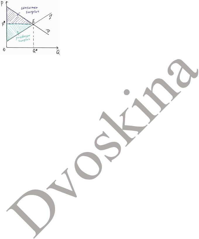
Market equilibrium results in largest total surplus

Buyer’s (consumer) surplus = difference between his reservation price and the price he actually pays.

Seller’s (producer) surplus = difference between the price he receives and his reservation price.

Elasticity

Price Elasticity of Demand

percentage change in quantity demanded/percentage change in price

| | = ∞= 0 | | > 1

| | = 1 − | | < 1

non-linear (relative to very small changes in price)

where P’(Q) is slope at the point ( ( ), )

arc

− 0

+ 0

2

− 0

+ 0

2

Total Expenditure = Revenue = P*Q(P)

Cross-price elasticity of demand – the percentage by which quantity demanded of the first good changes in response to a 1 percent change in the price of the second.

Substitutes >0, Complements <0

Income elasticity of demand – … 1 percent change in income. Normal good >0, inferior good <0

Price elasticity of supply

percentage change in quantity supplied that occurs in response to a 1 percent change in price

∆= ∆

always positive

Taxation

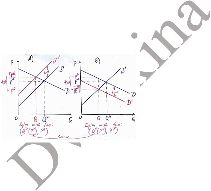
Per-unit tax is collected from sellers: equivalent to increase in marginal costs. Graphically – shift supply up by the amount of the tax.

Buyers pay: PB, Sellers get: PS=PB-tax. Quantity traded is QD(PB).

Per-unit tax is collected from buyers: equivalent to decrease in maximum willingness to pay per unit. Graphically – shift demand down by the amount of the tax.

Buyers pay: PB, Sellers get: PS=PB-tax. Quantity traded is QS(PS).

Incidence of a tax describes who eventually bears the burden of it. Depends on the relative elasticities of demand and supply.

Tax revenue: t*QD(PB)

To project the amount of tax revenue, need to know elasticities of both demand and supply.

Consumer choice

Best and affordable consumption bundle – combination of goods, which gives highest utility.

1 ≥ 0 quantity of good 11 > 0 price of good 11 ≥ 0 quantity of good 22 > 0 price of good 2

≥ 0 denote the amount of money our consumer has

Budget constraint (line) – a combination of quantities of goods 1 and 2 that the consumer can just afford: 1 1 + 2 2 =

Slope of the budget line – measures the rate at which the market is willing to substitute good 1 for good 2.

∆2= − ∆1

Budget set 1 1 + 2 2 ≤

If we change wealth, parallel; if we change prices, the same point

Completeness: Consumer can always make a choice between X and Y.

Transitivity: If X is preferred to Y, and Y is preferred to Z, then X is preferred to Z.

Monotonicity: More is preferred to less.

Diminishing MRS: If consumer has a lot of good 2, in general she would be willing to give up more of it for an extra unit of good 1, without changing her utility, then if she had less of good 2 to begin with.

Indifference curve – shows all the consumption bundles that consumer likes equally well.

With standard assumptions (rationality and “more is better”) optimal consumption bundle lies on the highest indifference curve that touches the budget constraint (all income is spent).

Utility function assigns a particular number to every consumption bundle. Higher values of utility indicate more preferred bundles.

A number in itself has no value. Particular preferences can be represented with lots of utility functions. A utility function represents given preference relationship as long as: utility function assigns higher values to consumption bundles with greater quantities of goods (assume monotonicity of preferences or that “more is better”); it preserves the rate at which consumer is willing to substitute one good for another (MRS).

Consumer’s optimal choice is the bundle at which MRS is equal to the slope of the budget constraint

= − 12

or the market trade-off is equal to the utility trade-off required to maintain constant utility

Consumers prefer balanced bundles to the ones with relatively much larger quantities of either good, the best bundle they can afford.

“Best bundle” – preferences represented by indifference curves “Can afford” – budget constraint.

Budget constraint is tangent to the indifference curve.