

MICRO reference
.pdfMarginal utility of good 1 – increase in total utility obtained by consuming a little more of good 1(relative to the change in good 1)
|
= |
(1+∆1, 2)− (1,2) |
= |
∆ ( 1,2) |
|
|||||
|
|
|
|
|||||||
1 |
|
|
∆ 1 |
|
|
|
∆ 1 |
|||
|
|
|
|
|
|
|||||
For very small ∆1 |
|
|
|
|
|
|
||||
|
= lim |
∆ (1, 2) |
= |
(1, 2) |
|
|||||
|
|
|
||||||||
1 |
∆1→0 |
∆ |
|
|
|
|||||
|
|
|
1 |
|
1 |
|
|
|||
Diminishing marginal utility – each extra unit of a good consumed, holding constant consumption of other goods, adds successively less to utility.
Change in total utility= 1 1 + 2 2 = 0
MRS shows the quantity of good 2 consumer must sacrifice to increase the consumption of good 1 without changing his level of satisfaction (utility).
|
linear = = − |
∆2 |
perfect substitutes |
|
|||||||||||||||
∆1 |
|
||||||||||||||||||
|
|
|
|
|
|
|
|
|
|
|
∆2( 1) |
|
|
||||||
|
non-linear = = − |
lim |
= ′( ) |
||||||||||||||||
|
|
|
|||||||||||||||||
|
|
|
|
|
|
|
|
|
|
∆1→0 |
∆1 |
2 |
1 |
||||||
|
|
|
|
|
|
|
|
|
|
|
|
||||||||
|
= |
2 |
= − |
1 |
= − |
|
1 |
|
or |
|
1 |
|
= |
2 |
|
|
|||
|
|
|
|
|
|
|
|
|
|||||||||||
|
|
|
1 |
|
|
|
|
|
|
|
|
||||||||
|
|
|
2 |
|
2 |
|
|
1 |
|
2 |
|
|
|
||||||
Results of consumer choice
Income expansion path – shows how the chosen bundle varies with consumer income levels, keeping all else fixed.
Engle curve – shows how consumption of particular good varies with income (all else fixed).

Effects of price change
Income effect (consumer can afford more/less of consumption bundles; positive for normal goods, negative for inferior goods) –own & -cross-price
Substitution effect (relative prices/slope of the BC change)
–own-price always negative, P&Q of good I move in opposite directions
–cross-price always positive, P&Q of good i move in the same direction Net effect=income effect+substitution effect
Normal good (own price change)
Price increase:
Substitution effect: decrease in quantity demanded (negative);
Income effect: decrease in quantity demanded (negative).
Total: decrease in quantity demanded
Price decrease:
Substitution effect: increase in quantity demanded (negative);
Income effect: increase in quantity demanded (negative).
Total: increase in quantity demanded.
Price and quantity demanded move in opposite directions:
Total effect is negative.
Normal good (cross-price effect)
Price increase:
Substitution effect: increase in quantity demanded (positive);
Income effect: decrease in quantity demanded of (negative). Price decrease:
Substitution effect: decrease in quantity demanded (positive);
Income effect: increase in quantity demanded of (negative).
Quantity and price change in opposite directions (cross-price elasticity is negative) if goods are complements;
Quantity and price change in same direction (cross-price elasticity is positive) if goods are substitutes.
Inferior good (own price change)
Price increase:
Substitution effect: decrease in quantity demanded (negative);
Income effect: increase in quantity demanded (positive). Price decrease:
Substitution effect: increase in quantity demanded (negative); Income effect: decrease in quantity demanded (positive).
Price and quantity demanded can move in opposite directions, most often negative or can move in same direction, positive, Giffen good
Inferior good (cross-price effect) Price increase:
Substituton effect: increase in quantity demanded (positive);
Income effect: increase in quantity demanded (positive).
Total effect is positive.
Price decrease:
Substitution effect: decrease in quantity demanded (positive);
Income effect: decrease in quantity demanded (positive).
Total effect is positive.
Total: Price and quantity demanded move in the same direction (positive cross-price elasticity, goods 1 and 2 are substitutes).


BDF: Ch. 6, 7, 8, 9, 10, 11
FB: Ch. 6, 8, 10 , 11, 14
"Competition Policy: Theory and Practice”, Ch. 1
Producer (firm) cares about costs and revenues
Economics costs=accounting costs (actual payments of a firm) + opportunity costs (amounts lost by not using the resource (labor or capital) in its best alternative use) Economic profit=revenue-economic costs
Accounting profit=revenue-accounting costs
Revenue
TR(Q)=P(Q)*Q
TR is highest when MR=0
Marginal revenue - increase in total revenue when output is increased by 1 unit or extra revenue from selling last unit-revenue lost selling existing units at lower price.
MR declines with more output, because it depends on demand. A firm can sell more output only if the price is lower.
MR = extra revenue from selling last unit–revenue lost selling existing units at lower price.
MR=const=P for a competitive firm
( ) = ( )
MR increases if demand increases.
P(Q)=a-bQ, then MR(Q)=a-2bQ
TR is the highest when MR=0
Cost
Technology - an input (or factor of production) - any good or service used to produce output.
main inputs: capital and labor
other inputs: land and entrepreneurship
Producer chooses among production techniques that are efficient – cannot produce given amount of output with fewer/less expensive inputs.
It’s cheaper to produce additional units: use better technology, gain from technology, gain from experience. After some output level, further increases in production are at higher MC. Firm is too large and difficult to manage, more administrative costs.
( ) = ( )
Marginal cost - increase in total cost when output increases by 1 unit.
( + ∆) = |
( +∆ )− ( ) |
or |
lim |
( + ∆) = |
( ) |
= ( ) |
|
|
|||||
|
∆ |
∆ →0 |
|
|
|
|
MC increases if costs of inputs increase or technology deteriorates.
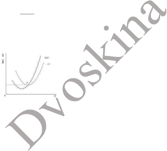
1)AC curve is first decreasing, then increasing
2)AC is declining whenever MC is below AC, and rising whenever MC is above AC
3)MC curve cuts the AC curve at the min. point of the AC curve

Relationships between values
The marginal product of a variable factor (labour) is the increase in output obtained by adding 1 unit of one variable factor, holding constant all other factors.
Diminishing marginal returns – relationship between changes in quantity of one input and output. Only one factor is varied, others are fixed at particular level.
The law of diminishing marginal returns: beyond some level of the variable input, further increases in the variable input lead to a steadily decreasing marginal product of this input.
Returns to scale – the quantitative change in output resulting from a proportionate increase in all inputs (long-run).
Multiply all factors by some positive constant t.
Increasing returns to scale: output increases more than t times.
Decreasing returns to scale: output increases less than t times.
Constant returns to scale (CRS): output increases exactly t times.
Economies (diseconomies) of scale - relationship between LAC and output. All factors can be varied.

Long-run
The long run is the period long enough for the firm to adjust all its inputs to a change in economic environment.
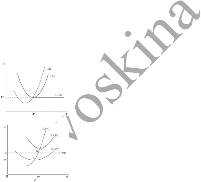
Choose quantity of output such that MR=LMC
If P(Q*)≥LAC(Q*) firm makes a profit, produce Q*; else: shutdown.
Short-run
The short run is the period in which the firm can make only partial adjustment of its inputs to a change in economic environment. We typically assume that capital is fixed in the short run. It takes up to several years to build a new plant.
Fixed costs are costs that do not vary with output level.
Variable costs are costs that vary with output level.
To maximize profit, choose quantitiy of output such that MR=SMC.
Fixed costs are sunk! Produce Q* as long as P(Q*)≥SAVC(Q*).
(A) profit, (B) loss (C) do not produce

Production decision
Produce additional units of output as long as MR≥MC.
Profit is highest where MR=MC.
Firm (Producer) makes decisions
1)whether it wants to be in the market AC<P
2)how much output to produce MR=MC
MR depends on market demand
Costs depend on technology and costs of inputs (firms choose efficient and cheapest technology to produce any given quantity of output → cost functions)
Shape of cost functions depends on properties of technology and input prices (economies/diseconomies of scale)
If firm is making a positive profit in the SR, in the LR it would increase its fixed factors of production to increase production of output.
If firm is making a loss in the SR, it should either contract its fixed factors in the LR or exit the market, depending on whether it can make a profit in the LR or not.

Market structure
“Artificial” factors:
exclusive control over important inputs
patents and copyrights
government licenses or franchises
“Natural” factors:
economies of scale
network economies
“Natural market structure”
The minimum efficient scale is the minimum output at which a firm’s long-run average cost curve stops declining.
The minimum efficient scale vis-à-vis the size of the market determines how many firms
“fit” in the industry.
The natural monopoly and the perfect competition are the two limiting cases. Monopolistic competition and oligopoly are the intermediate cases.
Perfect Competition
many buyers and sellers
many firms are producing the same good (and buyers know it is the same good)
no firm can affect the market price. firms are price-takers
demand curve is horizontal
firms can enter and exit freely
perfect information
can sell all it wants at market price P
can sell nothing at higher price
output decisions do not affect price: MR=P=D
demand curve is horizontal
TR(Q)=P*Q
MR(Q)=P
When the market price exceeds P*, a typical firm can make an economic profit. Hence many new firms will enter, and the price will fall back to P*.
SMC curve above point A is supply
To maximize profit, choose quantity of output such that MR=SMC P=SMC
Produce Q* as long as P*≥SAVC(Q*). Do not produce otherwise.