

MICRO reference
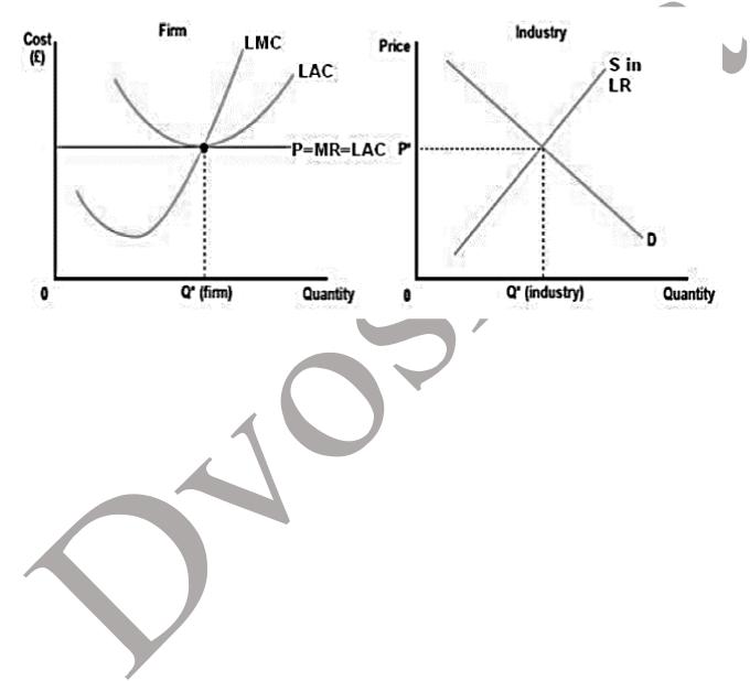
.pdfTo maximize profit, choose quantity of output such that MR=LMC P=LMC
Produce Q* as long as P*≥LAC(Q*)
Exit the market otherwise.
At any price above P* firm makes positive profit
AT P*, profit is 0: normal profit
If firm is making positive profit in the SR, in the LR it can add fixed inputs (build another factory, rent more space…) and increase output.
If price is low and firm is making negative profit (loss) in the SR, in the LR it may decrease its fixed inputs or exit the industry.
Entry: in perfect competition – free (long run decision), other new firms join industry when economic profit >0.
Thus, in equilibrium last firm that enters (marginal firm) has economic profit = 0.
Exit: Existing firms shut down when economic profit <0.
If firms have the same technology, then all firms make 0 profits.
Equilibrium
in competitive industry keeping all else fixed
SR: market price equates the quantity demanded to the total quantity supplied by the given number of firms in the industry when each firm produces on its short-run supply curve
LR: market price equates the quantity demanded to the total quantity supplied when each firm produces on its long-run supply curve, and the marginal firm makes only normal (zero) profits
Comparative statics for a competitive industry
Change some of the all else fixed: input prices or technology or prices of other goods or consumer incomes …
Model changes to the industry equilibrium in the SR and in the LR
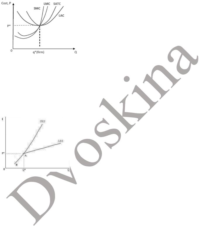
Firm when zero profits
Industry SRS = horizontal sum of the SRS curves of individual (existing) firms. Industry LRS = horizontal sum of the LRS curves of existing firms and firms that might potentially enter the industry.
LRS curve is flatter than the SRS curve.
at firm level: inputs are more flexible in the LR
at industry level: entry and exit, number of firms is flexible
Upward-sloping Supply curve
Many firms with possibly different costs
at P<P*, in the SR some firms make negative profits, but still produce
in the LR, marginal firm breaks even at P=P*, makes normal profit
higher price induces entry of less technologically efficient firms (with higher costs)
to produce more output firms demand more inputs → input prices increase with Q
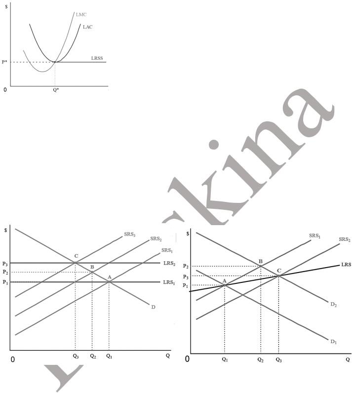
Constant AC (=min AC of individual firms)
all firms are identical
input costs do not change with output
output expands through entry of new firms
at any price above P* firms make supernormal (>0) profits → new firms enter →
price falls to P* unlikely
LMC (and LAC) depend on technology and input prices
technology differs by firm
input prices do not stay the same
Constant AC industry: effect of increase in input costs
Initial equilibrium: A
1)From A to B: reduce inputs and production in the SR: SRS2
2)In the LR, reduce fixed inputs, some firms exit: LRS2
3)SRS declines further to SRS3 due to further readjustment of inputs: New SR and LR eq’m in C.
Initial equilibrium: A
1)Increase in demand shifts the demand curve to the right (or up).
2)In the SR equilibrium moves from A to B. Q↑, P↑ Existing firms make economic profits >0.
3)In the long run existing firms expand their capital stock, new firms enter the
industry, SRS curve shifts down. The equilibrium moves from B to C. Q ↑, P ↓
Monopoly
1 large supplier (both current and potential)
maximize profit: MR=MC
firm’s downward-sloping demand curve coincides with the whole market demand curve
MR(Q)<P(Q), since P’(Q)<0: can sell an additional unit only by cutting price on all units
typically makes an economic profit in the short run and in the long-run (since no free entry)
MC>0 for all levels of output MR(Q)>0 when |ε| > 1
never produces on the inelastic part of the demand curve
economies of scale over the entire range of output
no supply curve as quantity produced depends on demand
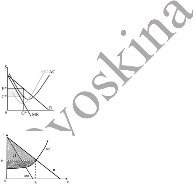
produce Q* if C*=AC(Q*) < P*
maximize profit if produce Q*: MC(Q*)=MR(Q*), charge P*=P(Q*)
welfare is highest with Qc such that Pс = MC (competitive output)
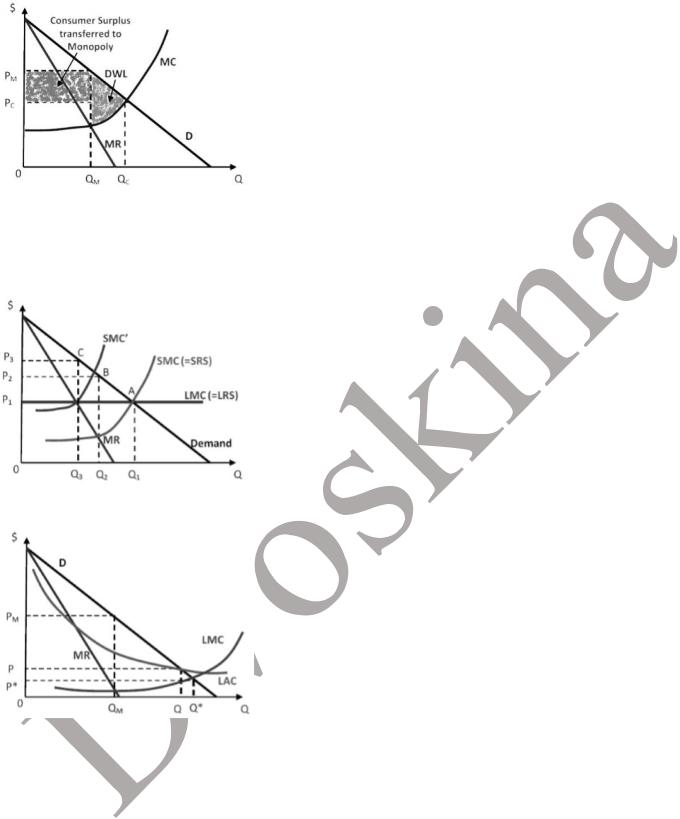
monopoly is inefficient: Qm < Qc
Monopoly vs. Efficiency: Two cases
Artificial Monopoly: Monopolization of competitive industry
constant ac competitive industry
produces Q1 where P=LMC=SMC for each firm monopoly takes over
in the SR produces Q2 where MR=SMC in the LR produces Q3 where MR=LMC deadweight loss.
regulate: break-up.
Natural Monopoly (large economies of scale or network economies)
meets the entire demand from a single plant monopolist chooses QM, where MR=LMC inefficient, DWL
Q* is efficient quantity (P=LMC) but: loss
if break-up, lose economies of scale
1)Order to produce Q at price P: cover LAC, smaller DWL
2)Order to produce Q* at price P*, cover losses via subsidy
3)Two-part tariff: per unit price P* plus fixed sum to cover the fixed costs.
Common carriage, open access: competing firms are allowed and pay to provide goods or services via the same infrastructure, provided by a regulated firm. Competitors pay for use of infrastructure.
Problems:
-Private monopoly: Cost are private information.
-State monopoly: Poor incentives to reduce costs.


Public Policy towards Monopoly
antitrust laws and state regulation (monopoly, merger control, pricing limitations, predatory practices)
state ownership
Price Discrimination
a discriminating monopoly can charge different prices to different consumers
1.1st degree (perfect price) discrimination
makes the MR curve coincide with demand curve (MRPD)
hurdle method of price discrimination – the practice by which a seller offers a discount to all buyers who overcome some obstacle (mail-in rebates, coupons, sales)
2.2nd degree price discrimination
price varies by quantity demanded. larger quantities are offered at a lower unit price.
3.3rd degree price discrimination
price varies by consumer attributes (location, segment) (student or senior discounts)
Price discrimination can be beneficial to both buyers and the monopolist: total surplus is larger.

good points
natural monopolies: production at lower average costs
potential profits provide incentives for r&d: patents and licenses
bad points
monopolist restricts output and drives up prices (bad)
it creates a deadweight loss (lower with price discrimination)
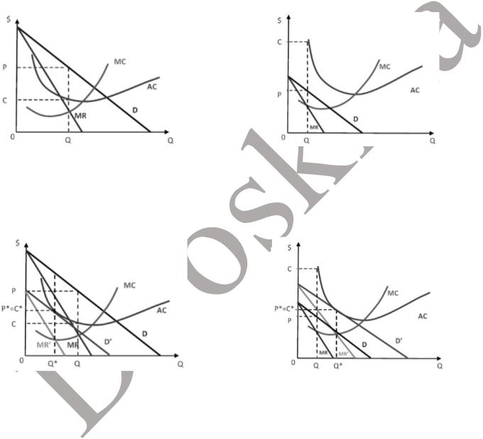
Monopolistic Competition
many sellers produce products that are close (but not perfect!) substitutes for one another
lots of small firms
downward-sloping demand curve for individual firm
product differentiation (brand, location)
free entry
zero profits (due to free entry)
In the short run this firm is making a profit: (P-C)Q>0
Potential entrants observe this and enter the industry. Thus, demand for firm’s product decreases.
In the short run this firm is making a loss: (P-C)Q<0
Firms exit the industry. Demand for products of remaining firms increases.
D falls to D’→MR falls to MR’. |
D increases to D’ → MR increases to |
Free entry: entry continues untill |
MR’. |
profits=0. |
Free entry: exit continues until profits=0 |
In the long run profit=0. |
for remaining firms. |
Q* is such that MR=MC. |
In the long run profit=0. |
P(Q*)=AC(Q*), that is, P*=C*. |
Q* is such that MR=MC. |
|
P(Q*)=AC(Q*), that is, P*=C*. |
Monopolistic Competition in the LR
1.firms are not producing at lowest point of AC curve (excess capacity);
2.price exceeds MC (monopoly power).
3.price = AC, zero profit.