

Mankiw Macroeconomics (5th ed)
.pdff i g u r e 1 6 - 1 0
Consumption, C
aW
C H A P T E R 1 6 Consumption | 449
The Life-Cycle Consumption Function The life-cycle model says that consumption depends on wealth as well as income. In other words, the intercept of the consumption function depends on wealth.
Income, Y
Notice, however, that the intercept of the consumption function, which shows what would happen to consumption if income ever fell to zero, is not a fixed value, as it is in Figure 16-1. Instead, the intercept here is aW and, thus, depends on the level of wealth.
This life-cycle model of consumer behavior can solve the consumption puzzle. According to the life-cycle consumption function, the average propensity to consume is
C/Y = a(W/Y ) + b.
Because wealth does not vary proportionately with income from person to person or from year to year, we should find that high income corresponds to a low average propensity to consume when looking at data across individuals or over short periods of time. But, over long periods of time, wealth and income grow together, resulting in a constant ratio W/Y and thus a constant average propensity to consume.
To make the same point somewhat differently, consider how the consumption function changes over time.As Figure 16-10 shows, for any given level of wealth, the life-cycle consumption function looks like the one Keynes suggested. But this function holds only in the short run when wealth is constant. In the long run, as wealth increases, the consumption function shifts upward, as in Figure 16-11. This upward shift prevents the average propensity to consume from falling as income increases. In this way, Modigliani resolved the consumption puzzle posed by Simon Kuznets’s data.
The life-cycle model makes many other predictions as well. Most important, it predicts that saving varies over a person’s lifetime. If a person begins adulthood with no wealth, she will accumulate wealth during her working
User SONPR:Job EFF01432:6264_ch16:Pg 449:28167#/eps at 100% *28167* |
Wed, Feb 20, 2002 3:13 PM |
|||
|
|
|
|
|
|
|
|
|
|
450 | P A R T V I More on the Microeconomics Behind Macroeconomics
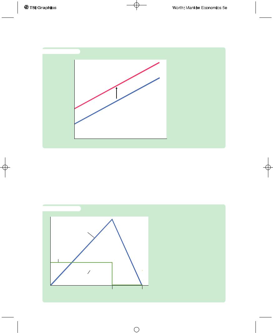
f i g u r e 1 6 - 1 1
Consumption, C
aW2
aW1
How Changes in Wealth Shift the Consumption Function If consumption depends on wealth, then an increase in wealth shifts the consumption function upward. Thus, the short-run consumption function (which holds wealth constant) will not continue to hold in the long run (as wealth rises over time).
Income, Y
years and then run down her wealth during her retirement years. Figure 16-12 illustrates the consumer’s income, consumption, and wealth over her adult life. According to the life-cycle hypothesis, because people want to smooth consumption over their lives, the young who are working save, while the old who are retired dissave.
f i g u r e 1 6 - 1 2
$
Consumption, Income, and Wealth Over the Life Cycle If the consumer smooths consumption over her life (as indicated by the horizontal consumption line), she will save and accumulate wealth during her working years and then dissave and run down her wealth during retirement.
|
|
|
|
|
|
|
|
Retirement |
End |
||
begins |
of life |
||
User SONPR:Job EFF01432:6264_ch16:Pg 450:28168#/eps at 100% *28168* |
Wed, Feb 20, 2002 3:13 PM |
|||
|
|
|
|
|
|
|
|
|
|

C H A P T E R 1 6 Consumption | 451
C A S E S T U D Y
The Consumption and Saving of the Elderly
Many economists have studied the consumption and saving of the elderly.Their findings present a problem for the life-cycle model. It appears that the elderly do not dissave as much as the model predicts. In other words, the elderly do not run down their wealth as quickly as one would expect if they were trying to smooth their consumption over their remaining years of life.
There are two chief explanations for why the elderly do not dissave to the extent that the model predicts. Each suggests a direction for further research on consumption.
The first explanation is that the elderly are concerned about unpredictable expenses. Additional saving that arises from uncertainty is called precautionary saving. One reason for precautionary saving by the elderly is the possibility of living longer than expected and thus having to provide for a longer than average span of retirement. Another reason is the possibility of illness and large medical bills.The elderly may respond to this uncertainty by saving more in order to be better prepared for these contingencies.
The precautionary-saving explanation is not completely persuasive, because the elderly can largely insure against these risks.To protect against uncertainty regarding life span, they can buy annuities from insurance companies. For a fixed fee, annuities offer a stream of income that lasts as long as the recipient lives. Uncertainty about medical expenses should be largely eliminated by Medicare, the government’s health insurance plan for the elderly, and by private insurance plans.
The second explanation for the failure of the elderly to dissave is that they may want to leave bequests to their children. Economists have proposed various theories of the parent–child relationship and the bequest motive. In Chapter 15 we discussed some of these theories and their implications for consumption and fiscal policy.
Overall, research on the elderly suggests that the simplest life-cycle model cannot fully explain consumer behavior.There is no doubt that providing for retirement is an important motive for saving, but other motives, such as precautionary saving and bequests, appear important as well.3
16-4 Milton Friedman and the
Permanent-Income Hypothesis
In a book published in 1957, Milton Friedman proposed the permanentincome hypothesis to explain consumer behavior. Friedman’s permanentincome hypothesis complements Modigliani’s life-cycle hypothesis: both use
3 To read more about the consumption and saving of the elderly, see Albert Ando and Arthur Kennickell,“How Much (or Little) Life Cycle Saving Is There in Micro Data?’’ in Rudiger Dornbusch, Stanley Fischer, and John Bossons, eds., Macroeconomics and Finance: Essays in Honor of Franco Modigliani
(Cambridge, Mass.: MIT Press, 1986); and Michael Hurd,“Research on the Elderly: Economic Status, Retirement, and Consumption and Saving,” Journal of Economic Literature 28 ( June 1990): 565–589.
User SONPR:Job EFF01432:6264_ch16:Pg 451:28169#/eps at 100% *28169* |
Wed, Feb 20, 2002 3:13 PM |
|||
|
|
|
|
|
|
|
|
|
|

452 | P A R T V I More on the Microeconomics Behind Macroeconomics
Irving Fisher’s theory of the consumer to argue that consumption should not depend on current income alone. But unlike the life-cycle hypothesis, which emphasizes that income follows a regular pattern over a person’s lifetime, the permanent-income hypothesis emphasizes that people experience random and temporary changes in their incomes from year to year.4
The Hypothesis
Friedman suggested that we view current income Y as the sum of two components, permanent income Y P and transitory income Y T.That is,
Y = Y P + Y T.
Permanent income is the part of income that people expect to persist into the future.Transitory income is the part of income that people do not expect to persist. Put differently, permanent income is average income, and transitory income is the random deviation from that average.
To see how we might separate income into these two parts, consider these examples:
Maria, who has a law degree, earned more this year than John, who is a high-school dropout. Maria’s higher income resulted from higher permanent income, because her education will continue to provide her a higher salary.
Sue, a Florida orange grower, earned less than usual this year because a freeze destroyed her crop. Bill, a California orange grower, earned more than usual because the freeze in Florida drove up the price of oranges.
Bill’s higher income resulted from higher transitory income, because he is no more likely than Sue to have good weather next year.
These examples show that different forms of income have different degrees of persistence. A good education provides a permanently higher income, whereas good weather provides only transitorily higher income.Although one can imagine intermediate cases, it is useful to keep things simple by supposing that there are only two kinds of income: permanent and transitory.
Friedman reasoned that consumption should depend primarily on permanent income, because consumers use saving and borrowing to smooth consumption in response to transitory changes in income. For example, if a person received a permanent raise of $10,000 per year, his consumption would rise by about as much. Yet if a person won $10,000 in a lottery, he would not consume it all in one year. Instead, he would spread the extra consumption over the rest of his life. Assuming an interest rate of zero and a remaining life span of 50 years,
4 Milton Friedman, A Theory of the Consumption Function (Princeton, N.J.: Princeton University Press, 1957).
User SONPR:Job EFF01432:6264_ch16:Pg 452:28170#/eps at 100% *28170* |
Wed, Feb 20, 2002 3:13 PM |
|||
|
|
|
|
|
|
|
|
|
|

C H A P T E R 1 6 Consumption | 453
consumption would rise by only $200 per year in response to the $10,000 prize. Thus, consumers spend their permanent income, but they save rather than spend most of their transitory income.
Friedman concluded that we should view the consumption function as approximately
C = aY P,
where a is a constant that measures the fraction of permanent income consumed. The permanent-income hypothesis, as expressed by this equation, states that consumption is proportional to permanent income.
Implications
The permanent-income hypothesis solves the consumption puzzle by suggesting that the standard Keynesian consumption function uses the wrong variable. According to the permanent-income hypothesis, consumption depends on permanent income; yet many studies of the consumption function try to relate consumption to current income. Friedman argued that this errors-in-variables problem explains the seemingly contradictory findings.
Let’s see what Friedman’s hypothesis implies for the average propensity to consume. Divide both sides of his consumption function by Y to obtain
APC = C/Y = aY P/Y.
According to the permanent-income hypothesis, the average propensity to consume depends on the ratio of permanent income to current income. When current income temporarily rises above permanent income, the average propensity to consume temporarily falls; when current income temporarily falls below permanent income, the average propensity to consume temporarily rises.
Now consider the studies of household data. Friedman reasoned that these data reflect a combination of permanent and transitory income. Households with high permanent income have proportionately higher consumption. If all variation in current income came from the permanent component, the average propensity to consume would be the same in all households. But some of the variation in income comes from the transitory component, and households with high transitory income do not have higher consumption. Therefore, researchers find that high-income households have, on average, lower average propensities to consume.
Similarly, consider the studies of time-series data. Friedman reasoned that year-to-year fluctuations in income are dominated by transitory income. Therefore, years of high income should be years of low average propensities to consume. But over long periods of time—say, from decade to decade—the variation in income comes from the permanent component. Hence, in long time-series, one should observe a constant average propensity to consume, as in fact Kuznets found.
User SONPR:Job EFF01432:6264_ch16:Pg 453:28171#/eps at 100% *28171* |
Wed, Feb 20, 2002 3:13 PM |
|||
|
|
|
|
|
|
|
|
|
|

454 | P A R T V I More on the Microeconomics Behind Macroeconomics
C A S E S T U D Y
The 1964 Tax Cut and the 1968 Tax Surcharge
The permanent-income hypothesis can help us to interpret how the economy responds to changes in fiscal policy. According to the IS–LM model of Chapters 10 and 11, tax cuts stimulate consumption and raise aggregate demand, and tax increases depress consumption and reduce aggregate demand. The permanent-income hypothesis, however, predicts that consumption responds only to changes in permanent income. Therefore, transitory changes in taxes will have only a negligible effect on consumption and aggregate demand. If a change in taxes is to have a large effect on aggregate demand, it must be permanent.
Two changes in fiscal policy—the tax cut of 1964 and the tax surcharge of 1968—illustrate this principle. The tax cut of 1964 was popular. It was announced to be a major and permanent reduction in tax rates. As we discussed in Chapter 10, this policy change had the intended effect of stimulating the economy.
The tax surcharge of 1968 arose in a very different political climate. It became law because the economic advisers of President Lyndon Johnson believed that the increase in government spending from theVietnam War had excessively stimulated aggregate demand.To offset this effect, they recommended a tax increase. But Johnson, aware that the war was already unpopular, feared the political repercussions of higher taxes. He finally agreed to a temporary tax surcharge—in essence, a one-year increase in taxes.The tax surcharge did not have the desired effect of reducing aggregate demand. Unemployment continued to fall, and inflation continued to rise.
The lesson to be learned from these episodes is that a full analysis of tax policy must go beyond the simple Keynesian consumption function; it must take into account the distinction between permanent and transitory income. If consumers expect a tax change to be temporary, it will have a smaller impact on consumption and aggregate demand.
16-5 Robert Hall and the Random-Walk
Hypothesis
The permanent-income hypothesis is based on Fisher’s model of intertemporal choice. It builds on the idea that forward-looking consumers base their consumption decisions not only on their current income but also on the income they expect to receive in the future. Thus, the permanent-income hypothesis highlights that consumption depends on people’s expectations.
Recent research on consumption has combined this view of the consumer with the assumption of rational expectations.The rational-expectations assumption states that people use all available information to make optimal forecasts
User SONPR:Job EFF01432:6264_ch16:Pg 454:28172#/eps at 100% *28172* |
Wed, Feb 20, 2002 3:13 PM |
|||
|
|
|
|
|
|
|
|
|
|

C H A P T E R 1 6 Consumption | 455
about the future. As we saw in Chapter 13, this assumption can have profound implications for the costs of stopping inflation. It can also have profound implications for the study of consumer behavior.
The Hypothesis
The economist Robert Hall was the first to derive the implications of rational expectations for consumption. He showed that if the permanent-income hypothesis is correct, and if consumers have rational expectations, then changes in consumption over time should be unpredictable.When changes in a variable are unpredictable, the variable is said to follow a random walk. According to Hall, the combination of the permanent-income hypothesis and rational expectations implies that consumption follows a random walk.
Hall reasoned as follows. According to the permanent-income hypothesis, consumers face fluctuating income and try their best to smooth their consumption over time. At any moment, consumers choose consumption based on their current expectations of their lifetime incomes. Over time, they change their consumption because they receive news that causes them to revise their expectations. For example, a person getting an unexpected promotion increases consumption, whereas a person getting an unexpected demotion decreases consumption. In other words, changes in consumption reflect “surprises” about lifetime income. If consumers are optimally using all available information, then they should be surprised only by events that were entirely unpredictable.Therefore, changes in their consumption should be unpredictable as well.5
Implications
The rational-expectations approach to consumption has implications not only for forecasting but also for the analysis of economic policies. If consumers obey the permanent-income hypothesis and have rational expectations, then only unexpected policy changes influence consumption.These policy changes take effect when they change expectations. For example, suppose that today Congress passes a tax increase to be effective next year. In this case, consumers receive the news about their lifetime incomes when Congress passes the law (or even earlier if the law’s passage was predictable). The arrival of this news causes consumers to revise their expectations and reduce their consumption.The following year, when the tax hike goes into effect, consumption is unchanged because no news has arrived.
Hence, if consumers have rational expectations, policymakers influence the economy not only through their actions but also through the public’s expectation of their actions. Expectations, however, cannot be observed directly.Therefore, it is often hard to know how and when changes in fiscal policy alter aggregate demand.
5 Robert E. Hall,“Stochastic Implications of the Life Cycle–Permanent Income Hypothesis:Theory and Evidence,’’ Journal of Political Economy 86 (April 1978): 971–987.
User SONPR:Job EFF01432:6264_ch16:Pg 455:28173#/eps at 100% *28173* |
Wed, Feb 20, 2002 3:13 PM |
|||
|
|
|
|
|
|
|
|
|
|

456 | P A R T V I More on the Microeconomics Behind Macroeconomics
C A S E S T U D Y
Do Predictable Changes in Income Lead to Predictable Changes in Consumption?
Of the many facts about consumer behavior, one is impossible to dispute: income and consumption fluctuate together over the business cycle.When the economy goes into a recession, both income and consumption fall, and when the economy booms, both income and consumption rise rapidly.
By itself, this fact doesn’t say much about the rational-expectations version of the permanent-income hypothesis. Most short-run fluctuations are unpredictable. Thus, when the economy goes into a recession, the typical consumer is receiving bad news about his lifetime income, so consumption naturally falls.And when the economy booms, the typical consumer is receiving good news, so consumption rises. This behavior does not necessarily violate the random-walk theory that changes in consumption are impossible to forecast.
Yet suppose we could identify some predictable changes in income. According to the random-walk theory, these changes in income should not cause consumers to revise their spending plans. If consumers expected income to rise or fall, they should have adjusted their consumption already in response to that information. Thus, predictable changes in income should not lead to predictable changes in consumption.
Data on consumption and income, however, appear not to satisfy this implication of the random-walk theory. When income is expected to fall by $1, consumption will on average fall at the same time by about $0.50. In other words, predictable changes in income lead to predictable changes in consumption that are roughly half as large.
Why is this so? One possible explanation of this behavior is that some consumers may fail to have rational expectations. Instead, they may base their expectations of future income excessively on current income.Thus, when income rises or falls (even predictably), they act as if they received news about their lifetime resources and change their consumption accordingly. Another possible explanation is that some consumers are borrowing-constrained and, therefore, base their consumption on current income alone. Regardless of which explanation is correct, Keynes’s original consumption function starts to look more attractive.That is, current income has a larger role in determining consumer spending than the random-walk hypothesis suggests.6
6 JohnY. Campbell and N. Gregory Mankiw,“Consumption, Income, and Interest Rates: Reinterpreting the Time-Series Evidence,” NBER Macroeconomics Annual (1989): 185–216; Jonathan Parker, “The Response of Household Consumption to Predictable Changes in Social Security Taxes,” American Economic Review 89 (September 1999): 959–973; and Nicholas S. Souleles, “The Response of Household Consumption to Income Tax Refunds,” American Economic Review 89 (September 1999): 947–958.
User SONPR:Job EFF01432:6264_ch16:Pg 456:28174#/eps at 100% *28174* |
Wed, Feb 20, 2002 3:13 PM |
|||
|
|
|
|
|
|
|
|
|
|

C H A P T E R 1 6 Consumption | 457
16.6David Laibson and the Pull of Instant Gratification
Keynes called the consumption function a “fundamental psychological law.”Yet, as we have seen, psychology has played little role in the subsequent study of consumption. Most economists assume that consumers are rational maximizers of utility who are always evaluating their opportunities and plans in order to obtain the highest lifetime satisfaction.This model of human behavior was the basis for all the work on consumption theory from Irving Fisher to Robert Hall.
More recently, economists have started to return to psychology. They have suggested that consumption decisions are not made by the ultrarational homo economicus but by real human beings whose behavior can be far from rational.The most prominent economist infusing psychology into the study of consumption is Harvard professor David Laibson.
Laibson notes that many consumers judge themselves to be imperfect decisionmakers. In one survey of the American public, 76 percent said they were not saving enough for retirement. In another survey of the baby-boom generation, respondents were asked the percentage of income that they save and the percentage that they thought they should save.The saving shortfall averaged 11 percentage points.
According to Laibson, the insufficiency of saving is related to another phenomenon: the pull of instant gratification. Consider the following two questions:
Question 1: Would you prefer (A) a candy today or (B) two candies tomorrow.
Question 2: Would you prefer (A) a candy in 100 days or (B) two candies in 101 days.
Many people confronted with such choices will answer A to the first question and B to the second. In a sense, they are more patient in the long run than they are in the short run.
This raises the possibility that consumers’ preferences may be time-inconsistent: they may alter their decisions simply because time passes. A person confronting question 2 may choose B and wait the extra day for the extra candy. But after 100 days pass, he then confronts question 1.The pull of instant gratification may induce him to change his mind.
We see this kind of behavior in many situations in life.A person on a diet may have a second helping at dinner, while promising himself that he will eat less tomorrow. A person may smoke one more cigarette, while promising himself that this is the last one. And a consumer may splurge at the shopping center, while promising himself that tomorrow he will cut back his spending and start saving more for retirement. But when tomorrow arrives, the promises are in the past, and a new self takes control of the decisionmaking, with its own desire for instant gratification.
These observations raise as many questions as they answer. Will the renewed focus on psychology among economists offer a better understanding of
User SONPR:Job EFF01432:6264_ch16:Pg 457:28175#/eps at 100% *28175* |
Wed, Feb 20, 2002 3:13 PM |
|||
|
|
|
|
|
|
|
|
|
|

458 | P A R T V I More on the Microeconomics Behind Macroeconomics
consumer behavior? Will it offer new prescriptions regarding, for instance, tax policy toward saving? It is too early to say, but without doubt, these questions are on the forefront of the research agenda.7
16.7 Conclusion
In the work of six prominent economists, we have seen a progression of views on consumer behavior. Keynes proposed that consumption depends largely on current income. Since then, economists have argued that consumers understand that they face an intertemporal decision. Consumers look ahead to their future resources and needs, implying a more complex consumption function than the one that Keynes proposed. Keynes suggested a consumption function of the form
Consumption = f (Current Income).
Recent work suggests instead that
Consumption
= f (Current Income,Wealth, Expected Future Income, Interest Rates).
In other words, current income is only one determinant of aggregate consumption. Economists continue to debate the importance of these determinants of consumption.There remains disagreement about, for example, the influence of interest rates on consumer spending, the prevalence of borrowing constraints, and the importance of psychological effects. Economists sometimes disagree about economic policy because they assume different consumption functions. For instance, as we saw in the previous chapter, the debate over the effects of government debt is in part a debate over the determinants of consumer spending.The key role of consumption in policy evaluation is sure to maintain economists’ interest in
studying consumer behavior for many years to come.
Summary
1.Keynes conjectured that the marginal propensity to consume is between zero and one, that the average propensity to consume falls as income rises, and that current income is the primary determinant of consumption. Studies of household data and short time-series confirmed Keynes’s conjectures. Yet studies of long time-series found no tendency for the average propensity to consume to fall as income rises over time.
2.Recent work on consumption builds on Irving Fisher’s model of the con-
sumer. In this model, the consumer faces an intertemporal budget constraint
7 For more on this topic, see David Laibson, “Golden Eggs and Hyperbolic Discounting,” Quarterly Journal of Economics 62 (May 1997): 443–477; and George-Marios Angeletos, David Laibson, Andrea Repetto, JeremyTobacman, and StephenWeinberg,“The Hyperbolic Buffer Stock Model: Calibration, Simulation, and Empirical Evidence,” Journal of Economic Perspectives, 15(3) (Summer 2001): 47–68.
User SONPR:Job EFF01432:6264_ch16:Pg 458:28176#/eps at 100% *28176* |
Wed, Feb 20, 2002 3:13 PM |
|||
|
|
|
|
|
|
|
|
|
|