

Mankiw Macroeconomics (5th ed)
.pdfC H A P T E R 1 1 Aggregate Demand II | 299
The Stabilizing Effects of Deflation In the IS–LM model we have developed so far, falling prices raise income. For any given supply of money M, a lower price level implies higher real money balances M/P. An increase in real money balances causes an expansionary shift in the LM curve, which leads to higher income.
Another channel through which falling prices expand income is called the Pigou effect. Arthur Pigou, a prominent classical economist in the 1930s, pointed out that real money balances are part of households’ wealth. As prices fall and real money balances rise, consumers should feel wealthier and spend more. This increase in consumer spending should cause an expansionary shift in the IS curve, also leading to higher income.
These two reasons led some economists in the 1930s to believe that falling prices would help stabilize the economy. That is, they thought that a decline in the price level would automatically push the economy back toward full employment.Yet other economists were less confident in the economy’s ability to correct itself. They pointed to other effects of falling prices, to which we now turn.
The Destabilizing Effects of Deflation Economists have proposed two theories to explain how falling prices could depress income rather than raise it.The first, called the debt-deflation theory, describes the effects of unexpected falls in the price level.The second explains the effects of expected deflation.
The debt-deflation theory begins with an observation from Chapter 4: unanticipated changes in the price level redistribute wealth between debtors and creditors. If a debtor owes a creditor $1,000, then the real amount of this debt is $1,000/P, where P is the price level.A fall in the price level raises the real amount of this debt—the amount of purchasing power the debtor must repay the creditor. Therefore, an unexpected deflation enriches creditors and impoverishes debtors.
The debt-deflation theory then posits that this redistribution of wealth affects spending on goods and services. In response to the redistribution from debtors to creditors, debtors spend less and creditors spend more. If these two groups have equal spending propensities, there is no aggregate impact. But it seems reasonable to assume that debtors have higher propensities to spend than creditors—perhaps that is why the debtors are in debt in the first place. In this case, debtors reduce their spending by more than creditors raise theirs.The net effect is a reduction in spending, a contractionary shift in the IS curve, and lower national income.
To understand how expected changes in prices can affect income, we need to add a new variable to the IS–LM model. Our discussion of the model so far has not distinguished between the nominal and real interest rates.Yet we know from previous chapters that investment depends on the real interest rate and that money demand depends on the nominal interest rate. If i is the nominal interest rate and pe is expected inflation, then the ex ante real interest rate is i − pe. We can now write the IS–LM model as
Y = C(Y − T ) + I(i − pe) + G |
IS, |
M/P = L(i, Y ) |
LM. |
Expected inflation enters as a variable in the IS curve.Thus, changes in expected inflation shift the IS curve.
User JOEWA:Job EFF01427:6264_ch11:Pg 299:27346#/eps at 100% *27346* |
Wed, Feb 13, 2002 10:27 AM |
|||
|
|
|
|
|
|
|
|
|
|
300 | P A R T I V Business Cycle Theory: The Economy in the Short Run
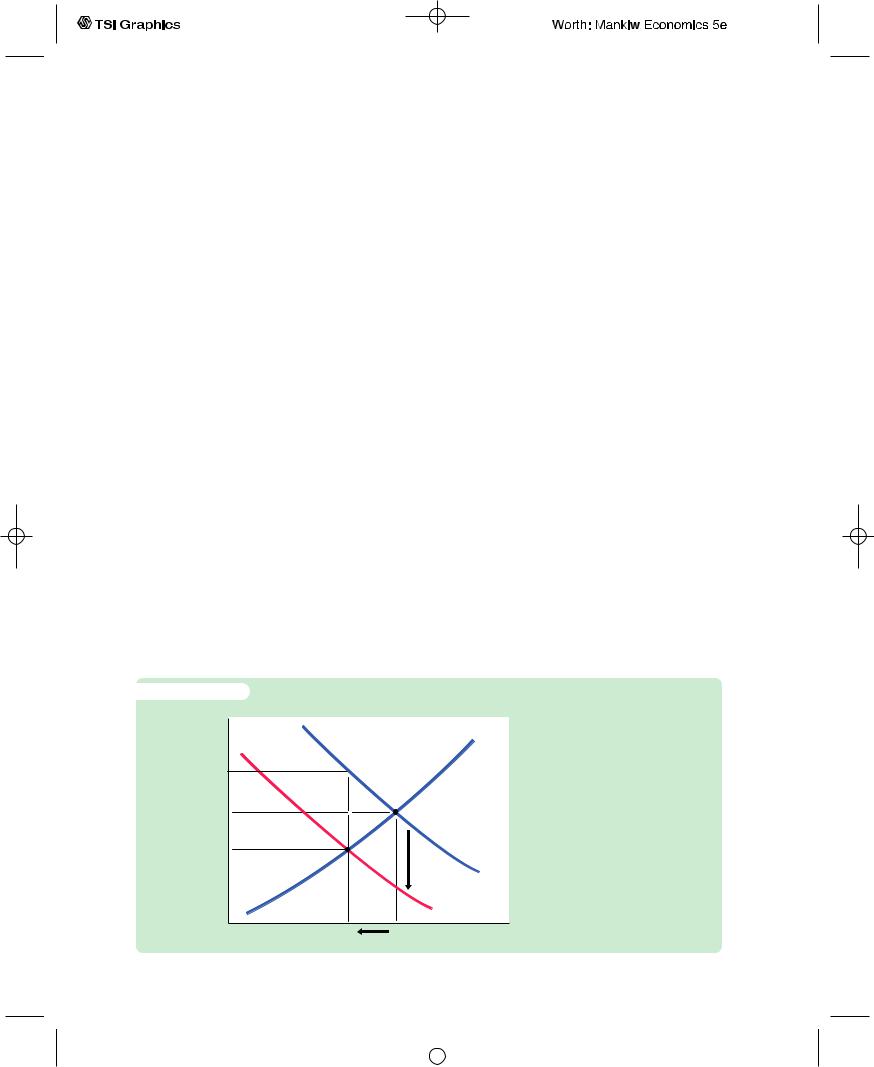
f i g u r e 1 1 - 8
Interest rate, i
r2
r1 i1
i2
Let’s use this extended IS–LM model to examine how changes in expected inflation influence the level of income.We begin by assuming that everyone expects the price level to remain the same. In this case, there is no expected inflation (pe = 0), and these two equations produce the familiar IS–LM model. Figure 11-8 depicts this initial situation with the LM curve and the IS curve labeled IS1. The intersection of these two curves determines the nominal and real interest rates, which for now are the same.
Now suppose that everyone suddenly expects that the price level will fall in the future, so that pe becomes negative. The real interest rate is now higher at any given nominal interest rate.This increase in the real interest rate depresses planned investment spending, shifting the IS curve from IS1 to IS2.Thus, an expected deflation leads to a reduction in national income from Y1 to Y2.The nominal interest rate falls from i1 to i2, whereas the real interest rate rises from r1 to r2.
Here is the story behind this figure. When firms come to expect deflation, they become reluctant to borrow to buy investment goods because they believe they will have to repay these loans later in more valuable dollars.The fall in investment depresses planned expenditure, which in turn depresses income. The fall in income reduces the demand for money, and this reduces the nominal interest rate that equilibrates the money market.The nominal interest rate falls by less than the expected deflation, so the real interest rate rises.
Note that there is a common thread in these two stories of destabilizing deflation. In both, falling prices depress national income by causing a contractionary shift in the IS curve. Because a deflation of the size observed from 1929 to 1933 is unlikely except in the presence of a major contraction in the money supply, these two explanations give some of the responsibility for the Depression—especially its severity—to the Fed. In other words, if falling prices are destabilizing, then a contraction in the money supply can lead to a fall in income, even without a decrease in real money balances or a rise in nominal interest rates.
|
Expected Deflation in the IS–LM |
|
Model An expected deflation (a |
|
negative value of pe) raises the |
|
real interest rate for any given |
|
nominal interest rate, and this |
|
depresses investment spending. |
|
The reduction in investment shifts |
|
the IS curve downward. The level |
|
of income falls from Y1 to Y2. The |
|
nominal interest rate falls from i1 |
|
to i2, and the real interest rate |
IS1 |
rises from r1 to r2. |
Y2 |
Y1 Income, output, Y |
User JOEWA:Job EFF01427:6264_ch11:Pg 300:27347#/eps at 100% *27347* |
Wed, Feb 13, 2002 10:27 AM |
|||
|
|
|
|
|
|
|
|
|
|

C H A P T E R 1 1 Aggregate Demand II | 301
Could the Depression Happen Again?
Economists study the Depression both because of its intrinsic interest as a major economic event and to provide guidance to policymakers so that it will not happen again. To state with confidence whether this event could recur, we would need to know why it happened. Because there is not yet agreement on the causes of the Great Depression, it is impossible to rule out with certainty another depression of this magnitude.
Yet most economists believe that the mistakes that led to the Great Depression are unlikely to be repeated.The Fed seems unlikely to allow the money supply to fall by one-fourth. Many economists believe that the deflation of the early 1930s was responsible for the depth and length of the Depression. And it seems likely that such a prolonged deflation was possible only in the presence of a falling money supply.
The fiscal-policy mistakes of the Depression are also unlikely to be repeated. Fiscal policy in the 1930s not only failed to help but actually further depressed aggregate demand. Few economists today would advocate such a rigid adherence to a balanced budget in the face of massive unemployment.
In addition, there are many institutions today that would help prevent the events of the 1930s from recurring. The system of Federal Deposit Insurance makes widespread bank failures less likely. The income tax causes an automatic reduction in taxes when income falls, which stabilizes the economy. Finally, economists know more today than they did in the 1930s. Our knowledge of how the economy works, limited as it still is, should help policymakers formulate better policies to combat such widespread unemployment.
C A S E S T U D Y
The Japanese Slump
During the 1990s, after many years of rapid growth and enviable prosperity, the Japanese economy experienced a prolonged downturn. Real GDP grew at an average rate of only 1.3 percent over the decade, compared with 4.3 percent over the previous twenty years.The unemployment rate, which had historically been very low in Japan, rose from 2.1 percent in 1990 to 4.7 percent in 1999. In August 2001, unemployment hit 5.0 percent, the highest rate since the government began compiling the statistic in 1953.
Although the Japanese slump of the 1990s is not even close in magnitude to the Great Depression of the 1930s, the episodes are similar in several ways. First, both episodes are traced in part to a large decline in stock prices. In Japan, stock prices at the end of the 1990s were less than half the peak level they had reached about a decade earlier. Like the stock market, Japanese land prices had also skyrocketed in the 1980s before crashing in the 1990s. (At the peak of Japan’s land bubble, it was said that the land under the Imperial Palace was worth more than the entire state of California.) When stock and land prices collapsed, Japanese citizens saw their wealth plummet.This decline in wealth, like that during the Great Depression, depressed consumer spending.
User JOEWA:Job EFF01427:6264_ch11:Pg 301:27348#/eps at 100% *27348* |
Wed, Feb 13, 2002 10:27 AM |
|||
|
|
|
|
|
|
|
|
|
|

302 | P A R T I V Business Cycle Theory: The Economy in the Short Run
Second, during both episodes, banks ran into trouble and exacerbated the slump in economic activity. Japanese banks in the 1980s had made many loans that were backed by stock or land. When the value of this collateral fell, borrowers started defaulting on their loans. These defaults on the old loans reduced the banks’ ability to make new loans. The resulting “credit crunch” made it harder for firms to finance investment projects and, thus, depressed investment spending.
Third, both episodes saw a fall in economic activity coincide with very low interest rates. In Japan in the 1990s, as in the United States in the 1930s, shortterm nominal interest rates were less than 1 percent. This fact suggests that the cause of the slump was primarily a contractionary shift in the IS curve, because such a shift reduces both income and the interest rate. The obvious suspects to explain the IS shift are the crashes in stock and land prices and the problems in the banking system.
Finally, the policy debate in Japan mirrored the debate over the Great Depression. Some economists recommended that the Japanese government pass large tax cuts to encourage more consumer spending. Although this advice was followed to some extent, Japanese policymakers were reluctant to enact very large tax cuts because, like the U.S. policymakers in the 1930s, they wanted to avoid budget deficits. In Japan, this reluctance to increase government debt arose in part because the government was facing a large unfunded pension liability and a rapidly aging population.
Other economists recommended that the Bank of Japan expand the money supply more rapidly. Even if nominal interest rates could not go much lower, then perhaps more rapid money growth could raise expected inflation, lower real interest rates, and stimulate investment spending. Thus, although economists differed about whether fiscal or monetary policy was more likely to be effective, there was wide agreement that the solution to Japan’s slump, like the solution to the Great Depression, rested in more aggressive expansion of aggregate demand.5
11-4 Conclusion
The purpose of this chapter and the previous one has been to deepen our understanding of aggregate demand. We now have the tools to analyze the effects of monetary and fiscal policy in the long run and in the short run. In the long run, prices are flexible, and we use the classical analysis of Parts II and III of this book. In the short run, prices are sticky, and we use the IS–LM model to examine how changes in policy influence the economy.
5 To learn more about this episode, see Adam S. Posen, Restoring Japan’s Economic Growth (Washington, DC: Institute for International Economics, 1998).
User JOEWA:Job EFF01427:6264_ch11:Pg 302:27349#/eps at 100% *27349* |
Wed, Feb 13, 2002 10:27 AM |
|||
|
|
|
|
|
|
|
|
|
|

C H A P T E R 1 1 Aggregate Demand II | 303
FYIThe Liquidity Trap
In Japan in the 1990s and the United States in the 1930s, interest rates reached very low levels. As Table 11-2 shows, U.S. interest rates were well under 1 percent throughout the second half of the 1930s. The same was true in Japan during the second half of the 1990s. In 1999, Japanese short-term interest rates fell to about one-tenth of 1 percent.
Some economists describe this situation as a liquidity trap. According to the IS–LM model, expansionary monetary policy works by reducing interest rates and stimulating investment spending. But if interest rates have already fallen almost to zero, then perhaps monetary policy is no longer effective. Nominal interest rates cannot fall below zero: rather than making a loan at a negative nominal interest rate, a person would simply hold cash. In this environment, expansionary monetary policy raises the supply of money, making the public more liquid, but because interest rates can’t fall any further, the extra liquidity might not have any effect. Aggregate demand, production, and employment may be “trapped” at low levels.
Other economists are skeptical about this argument. One response is that expansionary monetary policy might raise inflation expectations. Even if nominal interest rates cannot fall any further, higher expected inflation can lower real in-
terest rates by making them negative, which would stimulate investment spending. A second response is that monetary expansion would cause the currency to lose value in the market for foreign-currency exchange. This depreciation would make the nation’s goods cheaper abroad, stimulating export demand. This second argument goes beyond the closed-economy IS–LM model we have used in this chapter, but it has merit in the open-economy version of the model developed in the next chapter.
Is the liquidity trap something about which monetary policymakers need to worry? Might the tools of monetary policy at times lose their power to influence the economy? There is no consensus about the answers. Skeptics say we shouldn’t worry about the liquidity trap. But others say the possibility of a liquidity trap argues for a target rate of inflation greater than zero. Under zero inflation, the real interest rate, like the nominal interest, can never fall below zero. But if the normal rate of inflation is, say, 3 percent, then the central bank can easily push the real interest rate to negative 3 percent by lowering the nominal interest rate toward zero. Thus, moderate inflation gives monetary policymakers more room to stimulate the economy when needed, reducing the risk of falling into a liquidity trap.6
Although the model presented in this chapter provides the basic framework for analyzing aggregate demand, it is not the whole story. In later chapters, we examine in more detail the elements of this model and thereby refine our understanding of aggregate demand. In Chapter 16, for example, we study theories of consumption. Because the consumption function is a crucial piece of the IS–LM model, a deeper analysis of consumption may modify our view of the impact of monetary and fiscal policy on the economy.The simple IS–LM model presented in Chapters 10 and 11 provides the starting point for this further analysis.
6 To read more about the liquidity trap, see Paul R. Krugman, “It’s Baaack: Japan’s Slump and the Return of the Liquidity Trap,” Brookings Panel on Economic Activity (1998): 137–205.
User JOEWA:Job EFF01427:6264_ch11:Pg 303:27350#/eps at 100% *27350* |
Wed, Feb 13, 2002 10:27 AM |
|||
|
|
|
|
|
|
|
|
|
|

304 | P A R T I V Business Cycle Theory: The Economy in the Short Run
Summary
1.The IS–LM model is a general theory of the aggregate demand for goods and services.The exogenous variables in the model are fiscal policy, monetary policy, and the price level.The model explains two endogenous variables: the interest rate and the level of national income.
2.The IS curve represents the negative relationship between the interest rate and the level of income that arises from equilibrium in the market for goods and services.The LM curve represents a positive relationship between the interest rate and the level of income that arises from equilibrium in the market for real money balances. Equilibrium in the IS–LM model—the intersection of the IS and LM curves—represents simultaneous equilibrium in the market for goods and services and in the market for real money balances.
3.The aggregate demand curve summarizes the results from the IS–LM model by showing equilibrium income at any given price level. The aggregate demand curve slopes downward because a lower price level increases real money balances, lowers the interest rate, stimulates investment spending, and thereby raises equilibrium income.
4.Expansionary fiscal policy—an increase in government purchases or a decrease in taxes—shifts the IS curve to the right.This shift in the IS curve increases the interest rate and income. The increase in income represents a rightward shift in the aggregate demand curve. Similarly, contractionary fiscal policy shifts the IS curve to the left, lowers the interest rate and income, and shifts the aggregate demand curve to the left.
5. Expansionary monetary policy shifts the LM curve downward. This shift in the LM curve lowers the interest rate and raises income. The increase in income represents a rightward shift of the aggregate demand curve. Similarly, contractionary monetary policy shifts the LM curve upward, raises the interest rate, lowers income, and shifts the aggregate demand curve to the left.
K E Y C O N C E P T S
Monetary transmission mechanism |
Pigou effect |
Debt-deflation theory |
||
Q U E S T I O N S F O R R E V I E W |
|
|
|
|
|
|
|||
|
|
|
|
|
|
|
|
|
|
1.Explain why the aggregate demand curve slopes downward.
2.What is the impact of an increase in taxes on the interest rate, income, consumption, and investment?
3.What is the impact of a decrease in the money supply on the interest rate, income, consumption, and investment?
4.Describe the possible effects of falling prices on equilibrium income.
User JOEWA:Job EFF01427:6264_ch11:Pg 304:27351#/eps at 100% *27351* |
Wed, Feb 13, 2002 10:27 AM |
|||
|
|
|
|
|
|
|
|
|
|

C H A P T E R 1 1 Aggregate Demand II | 305
P R O B L E M S A N D A P P L I C A T I O N S
1.According to the IS–LM model, what happens to the interest rate, income, consumption, and investment under the following circumstances?
a.The central bank increases the money supply.
b.The government increases government purchases.
c.The government increases taxes.
d.The government increases government purchases and taxes by equal amounts.
2.Use the IS–LM model to predict the effects of each of the following shocks on income, the interest rate, consumption, and investment. In each case, explain what the Fed should do to keep income at its initial level.
shift? What are the new equilibrium interest rate and level of income?
e.Suppose instead that the money supply is raised from 1,000 to 1,200. How much does the LM curve shift? What are the new equilibrium interest rate and level of income?
f.With the initial values for monetary and fiscal policy, suppose that the price level rises from 2 to 4.What happens? What are the new equilibrium interest rate and level of income?
g.Derive and graph an equation for the aggregate demand curve. What happens to this aggregate demand curve if fiscal or monetary policy changes, as in parts (d) and (e)?
a.After the invention of a new high-speed computer chip, many firms decide to upgrade their computer systems.
b.A wave of credit-card fraud increases the frequency with which people make transactions in cash.
c.A best-seller titled Retire Rich convinces the public to increase the percentage of their income devoted to saving.
3.Consider the economy of Hicksonia.
a.The consumption function is given by
C = 200 + 0.75(Y − T ).
The investment function is
I = 200 − 25r.
Government purchases and taxes are both 100. For this economy, graph the IS curve for r ranging from 0 to 8.
b. The money demand function in Hicksonia is (M/P )d = Y − 100r.
The money supply M is 1,000 and the price level P is 2. For this economy, graph the LM curve for r ranging from 0 to 8.
c.Find the equilibrium interest rate r and the equilibrium level of income Y.
d.Suppose that government purchases are raised from 100 to 150. How much does the IS curve
4.Explain why each of the following statements is true. Discuss the impact of monetary and fiscal policy in each of these special cases.
a.If investment does not depend on the interest rate, the IS curve is vertical.
b.If money demand does not depend on the interest rate, the LM curve is vertical.
c.If money demand does not depend on income, the LM curve is horizontal.
d.If money demand is extremely sensitive to the interest rate, the LM curve is horizontal.
5.Suppose that the government wants to raise
investment but keep output constant. In the IS–LM model, what mix of monetary and fiscal policy will achieve this goal? In the early 1980s, the U.S. government cut taxes and ran a budget deficit while the Fed pursued a tight monetary policy. What effect should this policy mix have?
6.Use the IS–LM diagram to describe the shortrun and long-run effects of the following changes on national income, the interest rate, the price level, consumption, investment, and real money balances.
a.An increase in the money supply.
b.An increase in government purchases.
c.An increase in taxes.
User JOEWA:Job EFF01427:6264_ch11:Pg 305:27352#/eps at 100% *27352* |
Wed, Feb 13, 2002 10:28 AM |
|||
|
|
|
|
|
|
|
|
|
|

306 | P A R T I V Business Cycle Theory: The Economy in the Short Run
7.The Fed is considering two alternative monetary policies:
holding the money supply constant and letting the interest rate adjust, or
adjusting the money supply to hold the interest rate constant.
In the IS–LM model, which policy will better stabilize output under the following conditions?
a.All shocks to the economy arise from exogenous changes in the demand for goods and services.
b.All shocks to the economy arise from exogenous changes in the demand for money.
8.Suppose that the demand for real money balances depends on disposable income.That is, the money demand function is
M/P = L(r, Y − T ).
Using the IS–LM model, discuss whether this change in the money demand function alters the following:
a.The analysis of changes in government purchases.
b.The analysis of changes in taxes.
User JOEWA:Job EFF01427:6264_ch11:Pg 306:27353#/eps at 100% *27353* |
Wed, Feb 13, 2002 10:28 AM |
|||
|
|
|
|
|
|
|
|
|
|

C H A P T E R 1 1 Aggregate Demand II | 307
A P P E N D I X
The Simple Algebra of the IS–LM Model and the Aggregate Demand Curve
The chapter analyzes the IS–LM model with graphs of the IS and LM curves. Here we analyze the model algebraically rather than graphically.This alternative presentation offers additional insight into how monetary and fiscal policy influence aggregate demand.
The IS Curve
One way to think about the IS curve is that it describes the combinations of income Y and the interest rate r that satisfy an equation we first saw in Chapter 3:
Y = C(Y − T ) + I(r) + G.
This equation combines the national income accounts identity, the consumption function, and the investment function. It states that the quantity of goods produced, Y, must equal the quantity of goods demanded, C + I + G.
We can learn more about the IS curve by considering the special case in which the consumption function and investment function are linear. We begin with the national income accounts identity
Y = C + I + G.
Now suppose that the consumption function is
C = a + b(Y − T ),
where a and b are numbers greater than zero, and the investment function is
I = c − dr,
where c and d also are numbers greater than zero.The parameter b is the marginal propensity to consume, so we expect b to be between zero and one.The parameter d determines how much investment responds to the interest rate; because investment rises when the interest rate falls, there is a minus sign in front of d.
From these three equations, we can derive an algebraic expression for the IS curve and see what influences the IS curve’s position and slope. If we substitute the consumption and investment functions into the national income accounts identity, we obtain
Y = [a + b(Y − T )] + (c − dr) + G.
User JOEWA:Job EFF01427:6264_ch11:Pg 307:27354#/eps at 100% *27354* |
Wed, Feb 13, 2002 10:28 AM |
|||
|
|
|
|
|
|
|
|
|
|

308 | P A R T I V Business Cycle Theory: The Economy in the Short Run
Note that Y shows up on both sides of this equation.We can simplify this equation by bringing all the Y terms to the left-hand side and rearranging the terms on the right-hand side:
Y − bY = (a + c) + (G − bT ) − dr.
We solve for Y to get |
|
|
|
|
|
|
a + c |
|
1 |
|
−b |
|
−d |
Y = + G + T + r. |
||||||
1 − b |
1 |
− b |
1 |
− b |
1 |
− b |
This equation expresses the IS curve algebraically. It tells us the level of income Y for any given interest rate r and fiscal policy G and T. Holding fiscal policy fixed, the equation gives us a relationship between the interest rate and the level of income: the higher the interest rate, the lower the level of income. The IS curve graphs this equation for different values of Y and r given fixed values of G and T.
Using this last equation, we can verify our previous conclusions about the IS curve. First, because the coefficient of the interest rate is negative, the IS curve slopes downward: higher interest rates reduce income. Second, because the coefficient of government purchases is positive, an increase in government purchases shifts the IS curve to the right.Third, because the coefficient of taxes is negative, an increase in taxes shifts the IS curve to the left.
The coefficient of the interest rate, −d/(1 − b), tells us what determines whether the IS curve is steep or flat. If investment is highly sensitive to the interest rate, then d is large, and income is highly sensitive to the interest rate as well. In this case, small changes in the interest rate lead to large changes in income: the IS curve is relatively flat. Conversely, if investment is not very sensitive to the interest rate, then d is small, and income is also not very sensitive to the interest rate. In this case, large changes in interest rates lead to small changes in income: the IS curve is relatively steep.
Similarly, the slope of the IS curve depends on the marginal propensity to consume b.The larger the marginal propensity to consume, the larger the change in income resulting from a given change in the interest rate.The reason is that a large marginal propensity to consume leads to a large multiplier for changes in investment.The larger the multiplier, the larger the impact of a change in investment on income, and the flatter the IS curve.
The marginal propensity to consume b also determines how much changes in fiscal policy shift the IS curve.The coefficient of G, 1/(1 − b), is the govern- ment-purchases multiplier in the Keynesian cross. Similarly, the coefficient of T, −b/(1 − b), is the tax multiplier in the Keynesian cross. The larger the marginal propensity to consume, the greater the multiplier, and thus the greater the shift in the IS curve that arises from a change in fiscal policy.
The LM Curve
The LM curve describes the combinations of income Y and the interest rate r that satisfy the money market equilibrium condition
M/P = L(r, Y ).
User JOEWA:Job EFF01427:6264_ch11:Pg 308:27355#/eps at 100% *27355* |
Wed, Feb 13, 2002 10:28 AM |
|||
|
|
|
|
|
|
|
|
|
|