Mankiw Macroeconomics (5th ed)

part III

Growth Theory:

The Economy in

the Very Long Run

C H A P T E7R S E V E N

Economic Growth I

The question of growth is nothing new but a new disguise for an age-old

issue, one which has always intrigued and preoccupied economics: the

present versus the future.

— James Tobin

If you have ever spoken with your grandparents about what their lives were like when they were young, most likely you learned an important lesson about economics: material standards of living have improved substantially over time for most families in most countries. This advance comes from rising incomes, which have allowed people to consume greater quantities of goods and services.

To measure economic growth, economists use data on gross domestic product, which measures the total income of everyone in the economy. The real GDP of the United States today is more than three times its 1950 level, and real GDP per person is more than twice its 1950 level. In any given year, we can also observe large differences in the standard of living among countries. Table 7-1 shows income per person in 1999 of the world’s 12 most populous countries. The United States tops the list with an income of $31,910 per person. Nigeria has an income per person of only $770—less than 3 percent of the figure for the United States.

Our goal in this part of the book is to understand what causes these differences in income over time and across countries. In Chapter 3 we identified the factors of production—capital and labor—and the production technology as the sources of the economy’s output and, thus, of its total income. Differences in income, then, must come from differences in capital, labor, and technology.

Our primary task is to develop a theory of economic growth called the Solow growth model. Our analysis in Chapter 3 enabled us to describe how the economy produces and uses its output at one point in time. The analysis was static—a snapshot of the economy. To explain why our national income grows, and why some economies grow faster than others, we must broaden our analysis so that it describes changes in the economy over time. By developing such a model, we make our analysis dynamic—more like a movie than a photograph. The Solow growth model shows how saving, population growth, and

180 |

C H A P T E R 7 Economic Growth I | 181

t a b l e 7 - 1

International Differences in the Standard of Living: 1999

Source: World Bank.

technological progress affect the level of an economy’s output and its growth over time. In this chapter we analyze the roles of saving and population growth. In the next chapter we introduce technological progress.1

7-1 The Accumulation of Capital

The Solow growth model is designed to show how growth in the capital stock, growth in the labor force, and advances in technology interact in an economy, and how they affect a nation’s total output of goods and services. We build this model in steps. Our first step is to examine how the supply and demand for goods determine the accumulation of capital. In this first step, we assume that the labor force and technology are fixed.We then relax these assumptions by introducing changes in the labor force later in this chapter and by introducing changes in technology in the next.

The Supply and Demand for Goods

The supply and demand for goods played a central role in our static model of the closed economy in Chapter 3.The same is true for the Solow model. By considering the supply and demand for goods, we can see what determines how much output is produced at any given time and how this output is allocated among alternative uses.

1 The Solow growth model is named after economist Robert Solow and was developed in the 1950s and 1960s. In 1987 Solow won the Nobel Prize in economics for his work in economic growth.The model was introduced in Robert M. Solow, “A Contribution to the Theory of Economic Growth,’’ Quarterly Journal of Economics (February 1956): 65–94.

182 | P A R T I I I Growth Theory: The Economy in the Very Long Run

The Supply of Goods and the Production Function The supply of goods in the Solow model is based on the now-familiar production function, which states that output depends on the capital stock and the labor force:

Y = F(K, L).

The Solow growth model assumes that the production function has constant returns to scale. This assumption is often considered realistic, and as we will see shortly, it helps simplify the analysis. Recall that a production function has constant returns to scale if

zY = F(zK, zL)

for any positive number z.That is, if we multiply both capital and labor by z, we also multiply the amount of output by z.

Production functions with constant returns to scale allow us to analyze all quantities in the economy relative to the size of the labor force.To see that this is true, set z = 1/L in the preceding equation to obtain

Y/L = F(K/L, 1).

This equation shows that the amount of output per worker Y/L is a function of the amount of capital per worker K/L. (The number “1” is, of course, constant and thus can be ignored.) The assumption of constant returns to scale implies that the size of the economy—as measured by the number of workers—does not affect the relationship between output per worker and capital per worker.

Because the size of the economy does not matter, it will prove convenient to denote all quantities in per-worker terms.We designate these with lowercase letters, so y = Y/L is output per worker, and k = K/L is capital per worker.We can then write the production function as

y = f(k),

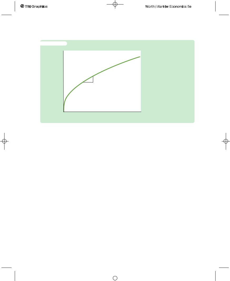
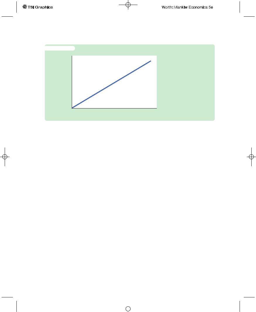
where we define f (k) = F(k,1). Figure 7-1 illustrates this production function. The slope of this production function shows how much extra output a worker

produces when given an extra unit of capital.This amount is the marginal product of capital MPK. Mathematically, we write

MPK = f (k + 1) − f (k).

Note that in Figure 7-1, as the amount of capital increases, the production function becomes flatter, indicating that the production function exhibits diminishing marginal product of capital. When k is low, the average worker has only a little capital to work with, so an extra unit of capital is very useful and produces a lot of additional output.When k is high, the average worker has a lot of capital, so an extra unit increases production only slightly.

The Demand for Goods and the Consumption Function The demand for goods in the Solow model comes from consumption and investment. In other

words, output per worker y is divided between consumption per worker c and investment per worker i:

y = c + i.

This equation is the per-worker version of the national income accounts identity for an economy. Notice that it omits government purchases (which for present purposes we can ignore) and net exports (because we are assuming a closed economy).

The Solow model assumes that each year people save a fraction s of their income and consume a fraction (1 − s).We can express this idea with a consumption function with the simple form

c = (1 − s)y,

where s, the saving rate, is a number between zero and one. Keep in mind that various government policies can potentially influence a nation’s saving rate, so one of our goals is to find what saving rate is desirable. For now, however, we just take the saving rate s as given.

To see what this consumption function implies for investment, substitute (1 − s)y for c in the national income accounts identity:

y = (1 − s)y + i.

Rearrange the terms to obtain

i = sy.

This equation shows that investment equals saving, as we first saw in Chapter 3. Thus, the rate of saving s is also the fraction of output devoted to investment.

184 | P A R T I I I Growth Theory: The Economy in the Very Long Run

We have now introduced the two main ingredients of the Solow model—the production function and the consumption function—which describe the economy at any moment in time. For any given capital stock k, the production function y = f (k) determines how much output the economy produces, and the saving rate s determines the allocation of that output between consumption and investment.

Growth in the Capital Stock and the Steady State

At any moment, the capital stock is a key determinant of the economy’s output, but the capital stock can change over time, and those changes can lead to economic growth. In particular, two forces influence the capital stock: investment and depreciation. Investment refers to the expenditure on new plant and equipment, and it causes the capital stock to rise. Depreciation refers to the wearing out of old capital, and it causes the capital stock to fall. Let’s consider each of these in turn.

As we have already noted, investment per worker i equals sy. By substituting the production function for y, we can express investment per worker as a function of the capital stock per worker:

i = sf(k).

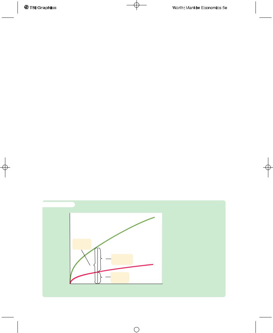
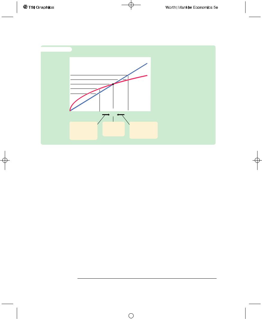
This equation relates the existing stock of capital k to the accumulation of new capital i. Figure 7-2 shows this relationship. This figure illustrates how, for any value of k, the amount of output is determined by the production function f (k), and the allocation of that output between consumption and saving is determined by the saving rate s.

To incorporate depreciation into the model, we assume that a certain fraction d of the capital stock wears out each year. Here d (the lowercase Greek letter delta) is called the depreciation rate. For example, if capital lasts an average of 25 years, then the depreciation rate is 4 percent per year (d = 0.04).The amount of capital that depreciates each year is dk. Figure 7-3 shows how the amount of depreciation depends on the capital stock.

We can express the impact of investment and depreciation on the capital stock with this equation:

Change in Capital Stock = Investment − Depreciation

Dk = i − dk,

where Dk is the change in the capital stock between one year and the next. Because investment i equals sf (k), we can write this as

Dk = sf(k) − dk.

Figure 7-4 graphs the terms of this equation—investment and depreciation—for different levels of the capital stock k.The higher the capital stock, the greater the amounts of output and investment.Yet the higher the capital stock, the greater also the amount of depreciation.

As Figure 7-4 shows, there is a single capital stock k* at which the amount of investment equals the amount of depreciation. If the economy ever finds itself at this level of the capital stock, the capital stock will not change because the two forces acting on it—investment and depreciation—just balance. That is, at k*, Dk = 0, so the capital stock k and output f (k) are steady over time (rather than growing or shrinking).We therefore call k* the steady-state level of capital.

The steady state is significant for two reasons. As we have just seen, an economy at the steady state will stay there. In addition, and just as important, an economy not at the steady state will go there.That is, regardless of the level of capital

186 | P A R T I I I Growth Theory: The Economy in the Very Long Run

f i g u r e 7 - 4

with which the economy begins, it ends up with the steady-state level of capital. In this sense, the steady state represents the long-run equilibrium of the economy.

To see why an economy always ends up at the steady state, suppose that the economy starts with less than the steady-state level of capital, such as level k1 in Figure 7-4. In this case, the level of investment exceeds the amount of depreciation. Over time, the capital stock will rise and will continue to rise—along with output f (k)—until it approaches the steady state k*.

Similarly, suppose that the economy starts with more than the steady-state level of capital, such as level k2. In this case, investment is less than depreciation: capital is wearing out faster than it is being replaced. The capital stock will fall, again approaching the steady-state level. Once the capital stock reaches the steady state, investment equals depreciation, and there is no pressure for the capital stock to either increase or decrease.

Approaching the Steady State: A Numerical Example

Let’s use a numerical example to see how the Solow model works and how the economy approaches the steady state. For this example, we assume that the production function is2

Y = K1/2L1/2.

2 If you read the appendix to Chapter 3, you will recognize this as the Cobb–Douglas production function with the parameter a equal to 1/2.

C H A P T E R 7 Economic Growth I | 187

To derive the per-worker production function f (k), divide both sides of the production function by the labor force L:

Because y = Y/L and k = K/L, this becomes

y = k1/2.

This equation can also be written as

y = k.

This form of the production function states that output per worker is equal to the square root of the amount of capital per worker.

To complete the example, let’s assume that 30 percent of output is saved (s = 0.3), that 10 percent of the capital stock depreciates every year (d = 0.1), and that the economy starts off with 4 units of capital per worker (k = 4). Given these numbers, we can now examine what happens to this economy over time.

We begin by looking at the production and allocation of output in the first year. According to the production function, the 4 units of capital per worker produce 2 units of output per worker. Because 30 percent of output is saved and invested and 70 percent is consumed, i = 0.6 and c = 1.4. Also, because 10 percent of the capital stock depreciates, dk = 0.4.With investment of 0.6 and depreciation of 0.4, the change in the capital stock is Dk = 0.2. The second year begins with 4.2 units of capital per worker.

Table 7-2 shows how the economy progresses year by year. Every year, new capital is added and output grows. Over many years, the economy approaches a steady state with 9 units of capital per worker. In this steady state, investment of 0.9 exactly offsets depreciation of 0.9, so that the capital stock and output are no longer growing.

Following the progress of the economy for many years is one way to find the steady-state capital stock, but there is another way that requires fewer calculations. Recall that

Dk = sf(k) − dk.

This equation shows how k evolves over time. Because the steady state is (by definition) the value of k at which Dk = 0, we know that

0 = sf (k*) − dk*,

or, equivalently,

k* s

= . f(k*) d

188 | P A R T I I I Growth Theory: The Economy in the Very Long Run

This equation provides a way of finding the steady-state level of capital per worker, k*. Substituting in the numbers and production function from our example, we obtain

k* 0.3= .k* 0.1

Now square both sides of this equation to find

k* = 9.

The steady-state capital stock is 9 units per worker.This result confirms the calculation of the steady state in Table 7-2.

C A S E S T U D Y

The Miracle of Japanese and German Growth

Japan and Germany are two success stories of economic growth.Although today they are economic superpowers, in 1945 the economies of both countries were in shambles. World War II had destroyed much of their capital stocks. In the