

Mankiw Macroeconomics (5th ed)
.pdfC H A P T E R 1 0 Aggregate Demand I | 279
2.Once we allow planned investment to depend on the interest rate, the Keynesian cross yields a relationship between the interest rate and national income. A higher interest rate lowers planned investment, and this in turn lowers national income.The downward-sloping IS curve summarizes this negative relationship between the interest rate and income.
3.The theory of liquidity preference is a basic model of the determination of the interest rate. It takes the money supply and the price level as exogenous and assumes that the interest rate adjusts to equilibrate the supply and demand for real money balances. The theory implies that increases in the money supply lower the interest rate.
4.Once we allow the demand for real money balances to depend on national income, the theory of liquidity preference yields a relationship between income and the interest rate. A higher level of income raises the demand for real money balances, and this in turn raises the interest rate.The upward-sloping LM curve summarizes this positive relationship between income and the interest rate.
5.The IS–LM model combines the elements of the Keynesian cross and the el-
ements of the theory of liquidity preference. The IS curve shows the points that satisfy equilibrium in the goods market, and the LM curve shows the points that satisfy equilibrium in the money market. The intersection of the IS and LM curves shows the interest rate and income that satisfy equilibrium in both markets.
K E Y C O N C E P T S
IS–LM model |
Keynesian cross |
Tax multiplier |
IS curve |
Government-purchases multiplier |
Theory of liquidity preference |
LM curve |
|
|
Q U E S T I O N S F O R R E V I E W
1.Use the Keynesian cross to explain why fiscal policy has a multiplied effect on national income.
2.Use the theory of liquidity preference to explain why an increase in the money supply lowers the
interest rate. What does this explanation assume about the price level?
3.Why does the IS curve slope downward?
4.Why does the LM curve slope upward?
P R O B L E M S A N D A P P L I C A T I O N S
1.Use the Keynesian cross to predict the impact of
a.An increase in government purchases.
b.An increase in taxes.
c.An equal increase in government purchases and taxes.
2.In the Keynesian cross, assume that the consumption function is given by
C = 200 + 0.75 (Y − T ).
Planned investment is 100; government purchases and taxes are both 100.
User JOEWA:Job EFF01426:6264_ch10:Pg 279:27288#/eps at 100% *27288* |
Wed, Feb 13, 2002 10:17 AM |
|||
|
|
|
|
|
|
|
|
|
|

280 | P A R T I V Business Cycle Theory: The Economy in the Short Run
a.Graph planned expenditure as a function of income.
b.What is the equilibrium level of income?
c.If government purchases increase to 125, what is the new equilibrium income?
d.What level of government purchases is needed to achieve an income of 1,600?
3.Although our development of the Keynesian cross in this chapter assumes that taxes are a fixed amount, in many countries (including the United States) taxes depend on income. Let’s represent the tax system by writing tax revenue as
−
where T and t are parameters of the tax code.The parameter t is the marginal tax rate: if income rises by $1, taxes rise by t × $1.
a.How does this tax system change the way consumption responds to changes in GDP?
b.In the Keynesian cross, how does this tax system alter the government-purchases multiplier?
c.In the IS–LM model, how does this tax system alter the slope of the IS curve?
4.Consider the impact of an increase in thriftiness in the Keynesian cross. Suppose the consumption
function is |
|
− |
+ c (Y − T ), |
C = C |
−
where C is a parameter called autonomous consump-
tion and c is the marginal propensity to consume.
a. What happens to equilibrium income when
the society becomes more thrifty, as repre-
−
sented by a decline in C
b.What happens to equilibrium saving?
c.Why do you suppose this result is called the paradox of thrift?
d.Does this paradox arise in the classical model of Chapter 3? Why or why not?
5.Suppose that the money demand function is
(M/P)d = 1,000 − 100r,
where r is the interest rate in percent.The money supply M is 1,000 and the price level P is 2.
a.Graph the supply and demand for real money balances.
b.What is the equilibrium interest rate?
c.Assume that the price level is fixed.What happens to the equilibrium interest rate if the supply of money is raised from 1,000 to 1,200?
d.If the Fed wishes to raise the interest rate to 7 percent, what money supply should it set?
User JOEWA:Job EFF01426:6264_ch10:Pg 280:27289#/eps at 100% *27289* |
Wed, Feb 13, 2002 10:18 AM |
|||
|
|
|
|
|
|
|
|
|
|

C H A P T1E R 1E L E V E N
Aggregate Demand II
Science is a parasite: the greater the patient population the better the ad-
vance in physiology and pathology; and out of pathology arises therapy.
The year 1932 was the trough of the great depression, and from its rotten
soil was belatedly begot a new subject that today we call macroeconomics.
— Paul Samuelson
In Chapter 10 we assembled the pieces of the IS–LM model.We saw that the IS curve represents the equilibrium in the market for goods and services, that the LM curve represents the equilibrium in the market for real money balances, and that the IS and LM curves together determine the interest rate and national income in the short run when the price level is fixed. Now we turn our attention to applying the IS–LM model to analyze three issues.
First, we examine the potential causes of fluctuations in national income.We use the IS–LM model to see how changes in the exogenous variables (government purchases, taxes, and the money supply) influence the endogenous variables (the interest rate and national income).We also examine how various shocks to the goods markets (the IS curve) and the money market (the LM curve) affect the interest rate and national income in the short run.
Second, we discuss how the IS–LM model fits into the model of aggregate supply and aggregate demand we introduced in Chapter 9. In particular, we examine how the IS–LM model provides a theory of the slope and position of the aggregate demand curve. Here we relax the assumption that the price level is fixed, and we show that the IS–LM model implies a negative relationship between the price level and national income. The model can also tell us what events shift the aggregate demand curve and in what direction.
Third, we examine the Great Depression of the 1930s.As this chapter’s opening quotation indicates, this episode gave birth to short-run macroeconomic theory, for it led Keynes and his many followers to think that aggregate demand was the key to understanding fluctuations in national income. With the benefit of hindsight, we can use the IS–LM model to discuss the various explanations of this traumatic economic downturn.
| 281
User JOEWA:Job EFF01427:6264_ch11:Pg 281:25874#/eps at 100% *25874* |
Wed, Feb 13, 2002 10:26 AM |
|||
|
|
|
|
|
|
|
|
|
|
282 | P A R T I V Business Cycle Theory: The Economy in the Short Run
11-1 Explaining Fluctuations With
the IS–LM Model
f i g u r e 1 1 - 1
Interest rate, r
r2
r1
3. . . . and the interest rate.
2. . . . which raises income . . .
The intersection of the IS curve and the LM curve determines the level of national income.When one of these curves shifts, the short-run equilibrium of the economy changes, and national income fluctuates. In this section we examine how changes in policy and shocks to the economy can cause these curves to shift.
How Fiscal Policy Shifts the IS Curve and
Changes the Short-Run Equilibrium
We begin by examining how changes in fiscal policy (government purchases and taxes) alter the economy’s short-run equilibrium. Recall that changes in fiscal policy influence planned expenditure and thereby shift the IS curve.The IS–LM model shows how these shifts in the IS curve affect income and the interest rate.
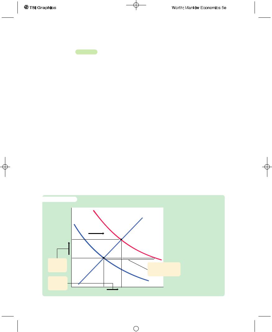
Changes in Government Purchases Consider an increase in government purchases of DG.The government-purchases multiplier in the Keynesian cross tells us that, at any given interest rate, this change in fiscal policy raises the level of income by DG/(1 − MPC).Therefore, as Figure 11-1 shows, the IS curve shifts to the right by this amount.The equilibrium of the economy moves from point A to point B. The increase in government purchases raises both income and the interest rate.
To understand fully what’s happening in Figure 11-1, it helps to keep in mind the building blocks for the IS–LM model from the preceding chapter—the Keynesian cross and the theory of liquidity preference. Here is the story. When the government
An Increase in Government Purchases in the IS–LM Model
An increase in government purchases shifts the IS curve to the right. The equilibrium moves from point A to point B. Income rises from Y1 to Y2, and the interest rate rises from r1 to r2.
1. The IS curve shifts to the right by
G/(1 MPC), . . .
IS1
Y1 |
Y2 |
Income, output, Y |
User JOEWA:Job EFF01427:6264_ch11:Pg 282:27329#/eps at 100% *27329* |
Wed, Feb 13, 2002 10:26 AM |
|||
|
|
|
|
|
|
|
|
|
|
C H A P T E R 1 1 Aggregate Demand II | 283
increases its purchases of goods and services, the economy’s planned expenditure rises.The increase in planned expenditure stimulates the production of goods and services, which causes total income Y to rise.These effects should be familiar from the Keynesian cross.
Now consider the money market, as described by the theory of liquidity preference. Because the economy’s demand for money depends on income, the rise in total income increases the quantity of money demanded at every interest rate. The supply of money has not changed, however, so higher money demand causes the equilibrium interest rate r to rise.
The higher interest rate arising in the money market, in turn, has ramifications back in the goods market.When the interest rate rises, firms cut back on their investment plans.This fall in investment partially offsets the expansionary effect of the increase in government purchases. Thus, the increase in income in response to a fiscal expansion is smaller in the IS–LM model than it is in the Keynesian cross (where investment is assumed to be fixed).You can see this in Figure 11-1. The horizontal shift in the IS curve equals the rise in equilibrium income in the Keynesian cross. This amount is larger than the increase in equilibrium income here in the IS–LM model.The difference is explained by the crowding out of investment caused by a higher interest rate.
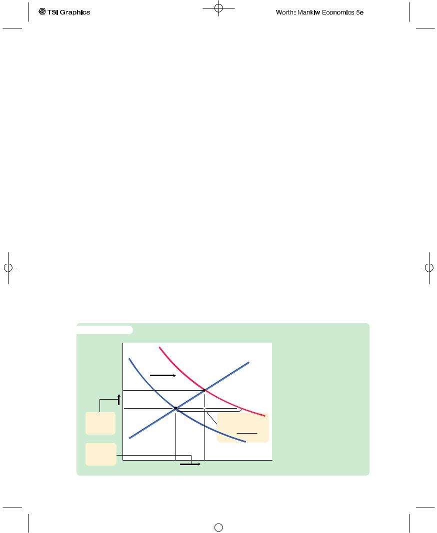
Changes in Taxes In the IS–LM model, changes in taxes affect the economy much the same as changes in government purchases do, except that taxes affect expenditure through consumption. Consider, for instance, a decrease in taxes of DT. The tax cut encourages consumers to spend more and, therefore, increases planned expenditure.The tax multiplier in the Keynesian cross tells us that, at any given interest rate, this change in policy raises the level of income by DT × MPC/(1 − MPC).Therefore, as Figure 11-2 illustrates, the IS curve shifts to the
f i g u r e 1 1 - 2 |
|
|
|
|
|
Interest rate, r |
|
|
|
|
|
r2 |
|
|
|
|
|
r1 |
|
|
|
IS |
2 |
3. . . . and |
|
|
|
|
|
|
1. The IS curve |
|
|
||
the interest |
|
shifts to the right by |
|||
rate. |
|
T |
MPC |
, . . . |
|
|
|
1 MPC |
|
|
|
2. . . . which |
|
|
IS1 |
|
|
raises |
|
|
|
|
|
income . . . |
Y2 |
Income, output, Y |
|||
Y1 |
|||||
A Decrease in Taxes in the
IS–LM Model A decrease in taxes shifts the IS curve to the right. The equilibrium moves from point A to point B. Income rises from Y1 to Y2, and the interest rate rises from r1 to r2.
User JOEWA:Job EFF01427:6264_ch11:Pg 283:27330#/eps at 100% *27330* |
Wed, Feb 13, 2002 10:26 AM |
|||
|
|
|
|
|
|
|
|
|
|
284 | P A R T I V Business Cycle Theory: The Economy in the Short Run
right by this amount. The equilibrium of the economy moves from point A to point B.The tax cut raises both income and the interest rate. Once again, because the higher interest rate depresses investment, the increase in income is smaller in the IS–LM model than it is in the Keynesian cross.
f i g u r e 1 1 - 3
Interest rate, r
r1
r2
3. . . . and lowers the interest rate.
2. . . . which raises income . . .
How Monetary Policy Shifts the LM Curve and Changes the Short-Run Equilibrium
We now examine the effects of monetary policy. Recall that a change in the money supply alters the interest rate that equilibrates the money market for any given level of income and, thereby, shifts the LM curve.The IS–LM model shows how a shift in the LM curve affects income and the interest rate.
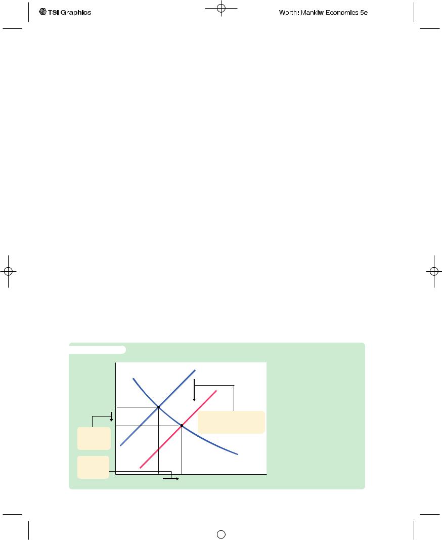
Consider an increase in the money supply. An increase in M leads to an increase in real money balances M/P, because the price level P is fixed in the short run.The theory of liquidity preference shows that for any given level of income, an increase in real money balances leads to a lower interest rate. Therefore, the LM curve shifts downward, as in Figure 11-3.The equilibrium moves from point A to point B.The increase in the money supply lowers the interest rate and raises the level of income.
Once again, to tell the story that explains the economy’s adjustment from point A to point B, we rely on the building blocks of the IS–LM model—the Keynesian cross and the theory of liquidity preference.This time, we begin with the money market, where the monetary-policy action occurs. When the Federal Reserve increases the supply of money, people have more money than they want to hold at the prevailing interest rate. As a result, they start depositing this extra money in banks or use it to buy bonds.The interest rate r then falls until people are willing to hold all the extra money that the Fed has created; this brings the money market to a new equilibrium.The lower interest rate, in turn,
LM1
LM2
1. An increase in the money supply shifts
the LM curve downward, . . .
An Increase in the Money Supply in the IS–LM Model
An increase in the money supply shifts the LM curve downward. The equilibrium moves from point A to point B. Income rises from Y1 to Y2, and the interest rate falls from r1 to r2.
|
|
IS |
Y1 |
Y2 |
Income, output, Y |
User JOEWA:Job EFF01427:6264_ch11:Pg 284:27331#/eps at 100% *27331* |
Wed, Feb 13, 2002 10:26 AM |
|||
|
|
|
|
|
|
|
|
|
|

C H A P T E R 1 1 Aggregate Demand II | 285
has ramifications for the goods market. A lower interest rate stimulates planned investment, which increases planned expenditure, production, and income Y.
Thus, the IS–LM model shows that monetary policy influences income by changing the interest rate.This conclusion sheds light on our analysis of monetary policy in Chapter 9. In that chapter we showed that in the short run, when prices are sticky, an expansion in the money supply raises income. But we did not discuss how a monetary expansion induces greater spending on goods and ser- vices—a process called the monetary transmission mechanism.The IS–LM model shows that an increase in the money supply lowers the interest rate, which stimulates investment and thereby expands the demand for goods and services.
The Interaction Between Monetary and Fiscal Policy
When analyzing any change in monetary or fiscal policy, it is important to keep in mind that the policymakers who control these policy tools are aware of what the other policymakers are doing. A change in one policy, therefore, may influence the other, and this interdependence may alter the impact of a policy change.
For example, suppose Congress were to raise taxes.What effect should this policy have on the economy? According to the IS–LM model, the answer depends on how the Fed responds to the tax increase.
Figure 11-4 shows three of the many possible outcomes. In panel (a), the Fed holds the money supply constant. The tax increase shifts the IS curve to the left. Income falls (because higher taxes reduce consumer spending), and the interest rate falls (because lower income reduces the demand for money). The fall in income indicates that the tax hike causes a recession.
In panel (b), the Fed wants to hold the interest rate constant. In this case, when the tax increase shifts the IS curve to the left, the Fed must decrease the money supply to keep the interest rate at its original level.This fall in the money supply shifts the LM curve upward.The interest rate does not fall, but income falls by a larger amount than if the Fed had held the money supply constant. Whereas in panel (a) the lower interest rate stimulated investment and partially offset the contractionary effect of the tax hike, in panel (b) the Fed deepens the recession by keeping the interest rate high.
In panel (c), the Fed wants to prevent the tax increase from lowering income. It must, therefore, raise the money supply and shift the LM curve downward enough to offset the shift in the IS curve. In this case, the tax increase does not cause a recession, but it does cause a large fall in the interest rate. Although the level of income is not changed, the combination of a tax increase and a monetary expansion does change the allocation of the economy’s resources. The higher taxes depress consumption, while the lower interest rate stimulates investment. Income is not affected because these two effects exactly balance.
From this example we can see that the impact of a change in fiscal policy depends on the policy the Fed pursues—that is, on whether it holds the money supply, the interest rate, or the level of income constant. More generally, whenever analyzing a change in one policy, we must make an assumption about its effect on the other policy. The most appropriate assumption depends on the case at hand and the many political considerations that lie behind economic policymaking.
User JOEWA:Job EFF01427:6264_ch11:Pg 285:27332#/eps at 100% *27332* |
Wed, Feb 13, 2002 10:26 AM |
|||
|
|
|
|
|
|
|
|
|
|

f i g u r e 1 1 - 4
(a) Fed Holds Money Supply Constant
Interest rate, r
1. A tax increase shifts the IS curve . . .
2. . . . but because the Fed holds the money supply constant, the LM curve LM stays the same.
IS1
IS2
Income, output, Y
(b) Fed Holds Interest Rate Constant
Interest rate, r
1. A tax increase shifts the IS curve . . .
2. . . . and to hold the interest rate constant, the Fed contracts the money supply.
LM2
LM1
IS1
IS2
Income, output, Y
Interest rate, r
1. A tax increase shifts the IS curve . . .
(c) Fed Holds Income Constant
2. . . . and to hold income constant, the Fed expands the money supply.
LM1
LM2
IS1
IS2
Income, output, Y
The Response of the Economy to a Tax Increase How the economy responds to a tax increase depends on how the monetary authority responds. In panel
(a) the Fed holds the money supply constant. In panel (b) the Fed holds the interest rate constant by reducing the money supply. In panel (c) the Fed holds the level of income constant by raising the money supply.
User JOEWA:Job EFF01427:6264_ch11:Pg 286:27333#/eps at 100% *27333* |
Wed, Feb 13, 2002 10:27 AM |
|||
|
|
|
|
|
|
|
|
|
|

C H A P T E R 1 1 Aggregate Demand II | 287
C A S E S T U D Y
Policy Analysis With Macroeconometric Models
The IS–LM model shows how monetary and fiscal policy influence the equilibrium level of income.The predictions of the model, however, are qualitative, not quantitative. The IS–LM model shows that increases in government purchases raise GDP and that increases in taxes lower GDP. But when economists analyze specific policy proposals, they need to know not only the direction of the effect but also the size. For example, if Congress increases taxes by $100 billion and if monetary policy is not altered, how much will GDP fall? To answer this question, economists need to go beyond the graphical representation of the IS–LM model.
Macroeconometric models of the economy provide one way to evaluate policy proposals. A macroeconometric model is a model that describes the economy quantitatively, rather than only qualitatively. Many of these models are essentially more complicated and more realistic versions of our IS–LM model. The economists who build macroeconometric models use historical data to estimate parameters such as the marginal propensity to consume, the sensitivity of investment to the interest rate, and the sensitivity of money demand to the interest rate. Once a model is built, economists can simulate the effects of alternative policies with the help of a computer.
Table 11-1 shows the fiscal-policy multipliers implied by one widely used macroeconometric model, the Data Resources Incorporated (DRI) model, named for the economic forecasting firm that developed it.The multipliers are given for two assumptions about how the Fed might respond to changes in fiscal policy.
One assumption about monetary policy is that the Fed keeps the nominal interest rate constant.That is, when fiscal policy shifts the IS curve to the right or to the left, the Fed adjusts the money supply to shift the LM curve in the same direction. Because there is no crowding out of investment due to a changing interest rate, the fiscal-policy multipliers are similar to those from the Keynesian cross.The DRI model indicates that, in this case, the government-purchases multiplier is 1.93, and the tax multiplier is −1.19. That is, a $100 billion increase in government purchases raises GDP by $193 billion, and a $100 billion increase in taxes lowers GDP by $119 billion.
t a b l e 1 1 - 1
The Fiscal-Policy Multipliers in the DRI Model
|
VALUE OF MULTIPLIERS |
|
|
|
|
Assumption About Monetary Policy |
DY/DG |
DY/DT |
Nominal interest rate held constant |
1.93 |
−1.19 |
Money supply held constant |
0.60 |
−0.26 |
Note: This table gives the fiscal-policy multipliers for a sustained change in government purchases or in personal income taxes. These multipliers are for the fourth quarter after the policy change is made.
Source: Otto Eckstein, The DRI Model of the U.S. Economy (New York: McGraw-Hill, 1983), 169.
User JOEWA:Job EFF01427:6264_ch11:Pg 287:27334#/eps at 100% *27334* |
Wed, Feb 13, 2002 10:27 AM |
|||
|
|
|
|
|
|
|
|
|
|

288 | P A R T I V Business Cycle Theory: The Economy in the Short Run
The second assumption about monetary policy is that the Fed keeps the money supply constant so that the LM curve does not shift. In this case, the interest rate rises, and investment is crowded out, so the multipliers are much smaller. The government-purchases multiplier is only 0.60, and the tax multiplier is only −0.26.That is, a $100 billion increase in government purchases raises GDP by $60 billion, and a $100 billion increase in taxes lowers GDP by $26 billion.
Table 11-1 shows that the fiscal-policy multipliers are very different under the two assumptions about monetary policy.The impact of any change in fiscal policy depends crucially on how the Fed responds to that change.
Shocks in the IS–LM Model
Because the IS–LM model shows how national income is determined in the short run, we can use the model to examine how various economic disturbances affect income. So far we have seen how changes in fiscal policy shift the IS curve and how changes in monetary policy shift the LM curve. Similarly, we can group other disturbances into two categories: shocks to the IS curve and shocks to the LM curve.
Shocks to the IS curve are exogenous changes in the demand for goods and services. Some economists, including Keynes, have emphasized that such changes in demand can arise from investors’ animal spirits—exogenous and perhaps selffulfilling waves of optimism and pessimism. For example, suppose that firms become pessimistic about the future of the economy and that this pessimism causes them to build fewer new factories.This reduction in the demand for investment goods causes a contractionary shift in the investment function: at every interest rate, firms want to invest less.The fall in investment reduces planned expenditure and shifts the IS curve to the left, reducing income and employment.This fall in equilibrium income in part validates the firms’ initial pessimism.
Shocks to the IS curve may also arise from changes in the demand for consumer goods. Suppose, for instance, that the election of a popular president increases consumer confidence in the economy.This induces consumers to save less for the future and consume more today.We can interpret this change as an upward shift in the consumption function. This shift in the consumption function increases planned expenditure and shifts the IS curve to the right, and this raises income.
Dist. by Universal Press Syndicate.
Calvin and Hobbes © 1992 Watterson.
User JOEWA:Job EFF01427:6264_ch11:Pg 288:27335#/eps at 100% *27335* |
Wed, Feb 13, 2002 10:27 AM |
|||
|
|
|
|
|
|
|
|
|
|