Mankiw Macroeconomics (5th ed)

C H A P T E R 1 0 Aggregate Demand I | 259

demand, it is the variable that links the two halves of the IS–LM model. The model shows how interactions between these markets determine the position and slope of the aggregate demand curve and, therefore, the level of national income in the short run.1

10-1 The Goods Market and the IS Curve

The IS curve plots the relationship between the interest rate and the level of income that arises in the market for goods and services. To develop this relationship, we start with a basic model called the Keynesian cross.This model is the simplest interpretation of Keynes’s theory of national income and is a building block for the more complex and realistic IS–LM model.

The Keynesian Cross

In The General Theory, Keynes proposed that an economy’s total income was, in the short run, determined largely by the desire to spend by households, firms, and the government.The more people want to spend, the more goods and services firms can sell.The more firms can sell, the more output they will choose to produce and the more workers they will choose to hire.Thus, the problem during recessions and depressions, according to Keynes, was inadequate spending. The Keynesian cross is an attempt to model this insight.

Planned Expenditure We begin our derivation of the Keynesian cross by drawing a distinction between actual and planned expenditure. Actual expenditure is the amount households, firms, and the government spend on goods and services, and as we first saw in Chapter 2, it equals the economy’s gross domestic product (GDP). Planned expenditure is the amount households, firms, and the government would like to spend on goods and services.

Why would actual expenditure ever differ from planned expenditure? The answer is that firms might engage in unplanned inventory investment because their sales do not meet their expectations. When firms sell less of their product than they planned, their stock of inventories automatically rises; conversely, when firms sell more than planned, their stock of inventories falls. Because these unplanned changes in inventory are counted as investment spending by firms, actual expenditure can be either above or below planned expenditure.

Now consider the determinants of planned expenditure. Assuming that the economy is closed, so that net exports are zero, we write planned expenditure E as the sum of consumption C, planned investment I, and government purchases G:

E = C + I + G.

1 The IS–LM model was introduced in a classic article by the Nobel-Prize-winning economist John R. Hicks, “Mr. Keynes and the Classics: A Suggested Interpretation,’’ Econometrica 5 (1937): 147–159.

260 | P A R T I V Business Cycle Theory: The Economy in the Short Run

To this equation, we add the consumption function

C = C(Y − T ).

This equation states that consumption depends on disposable income (Y − T ), which is total income Y minus taxes T.To keep things simple, for now we take planned investment as exogenously fixed:

I = I−.

And as in Chapter 3, we assume that fiscal policy—the levels of government purchases and taxes—is fixed:

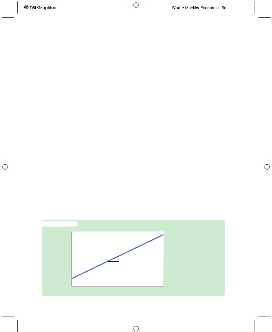
Figure 10-2 graphs planned expenditure as a function of the level of income. This line slopes upward because higher income leads to higher consumption and thus higher planned expenditure.The slope of this line is the marginal propensity to consume, the MPC: it shows how much planned expenditure increases when income rises by $1. This planned-expenditure function is the first piece of the model called the Keynesian cross.

The Economy in Equilibrium The next piece of the Keynesian cross is the assumption that the economy is in equilibrium when actual expenditure equals planned expenditure. This assumption is based on the idea that when people’s plans have been realized, they have no reason to change what they are doing.

Income, output, Y

C H A P T E R 1 0 Aggregate Demand I | 261

Recalling that Y as GDP equals not only total income but also total actual expenditure on goods and services, we can write this equilibrium condition as

Actual Expenditure = Planned Expenditure

Y = E.

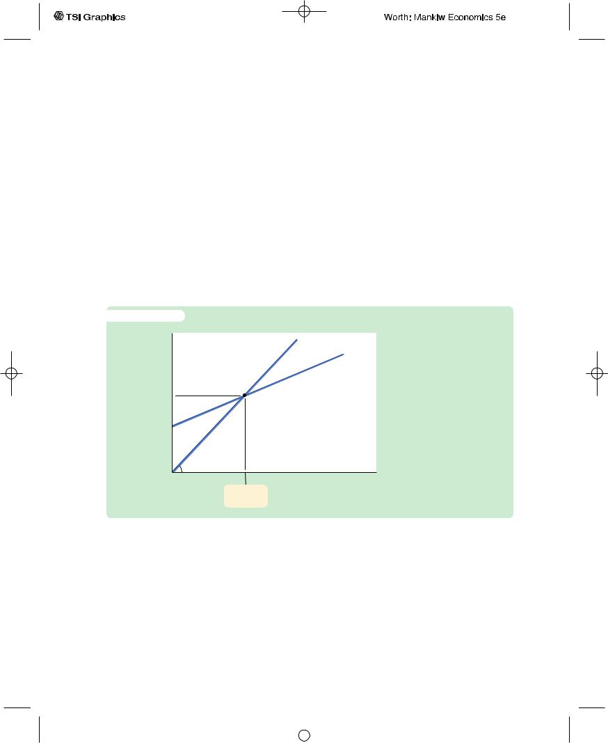
The 45-degree line in Figure 10-3 plots the points where this condition holds. With the addition of the planned-expenditure function, this diagram becomes the Keynesian cross. The equilibrium of this economy is at point A, where the planned-expenditure function crosses the 45-degree line.

How does the economy get to the equilibrium? In this model, inventories play an important role in the adjustment process.Whenever the economy is not in equilibrium, firms experience unplanned changes in inventories, and this induces them to change production levels. Changes in production in turn influence total income and expenditure, moving the economy toward equilibrium.

Income, output, Y

Equilibrium income

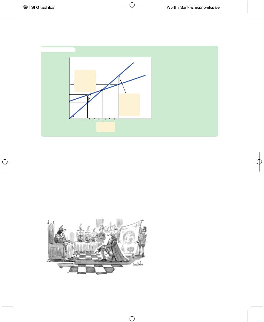
For example, suppose the economy were ever to find itself with GDP at a level greater than the equilibrium level, such as the level Y1 in Figure 10-4. In this case, planned expenditure E1 is less than production Y1, so firms are selling less than they are producing. Firms add the unsold goods to their stock of inventories. This unplanned rise in inventories induces firms to lay off workers and reduce production, and these actions in turn reduce GDP.This process of unintended inventory accumulation and falling income continues until income Y falls to the equilibrium level.

Similarly, suppose GDP were at a level lower than the equilibrium level, such as the level Y2 in Figure 10-4. In this case, planned expenditure E2 is greater than production Y2. Firms meet the high level of sales by drawing down their inventories.

262 | P A R T I V Business Cycle Theory: The Economy in the Short Run

But when firms see their stock of inventories dwindle, they hire more workers and increase production. GDP rises, and the economy approaches the equilibrium.

In summary, the Keynesian cross shows how income Y is determined for given levels of planned investment I and fiscal policy G and T. We can use this model to show how income changes when one of these exogenous variables changes.

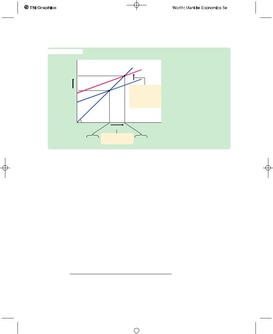
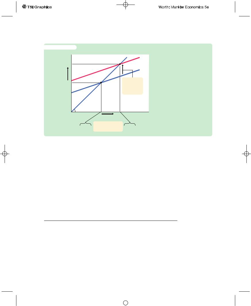
Fiscal Policy and the Multiplier: Government Purchases Consider how changes in government purchases affect the economy. Because government purchases are one component of expenditure, higher government purchases result in higher planned expenditure for any given level of income. If government purchases rise by DG, then the planned-expenditure schedule shifts upward by DG, as in Figure 10-5.The equilibrium of the economy moves from point A to point B.

The reason is that, according to the consumption function C = C(Y − T ), higher income causes higher consumption.When an increase in government purchases raises income, it also raises consumption, which further raises income, which further raises consumption, and so on.Therefore, in this model, an increase in government purchases causes a greater increase in income.

How big is the multiplier? To answer this question, we trace through each step of the change in income. The process begins when expenditure rises by DG, which implies that income rises by DG as well.This increase in income in turn raises consumption by MPC × DG, where MPC is the marginal propensity to consume. This increase in consumption raises expenditure and income once again.This second increase in income of MPC × DG again raises consumption, this time by MPC × (MPC × DG), which again raises expenditure and income, and so on.This feedback from consumption to income to consumption continues indefinitely.The total effect on income is

DY = (1 + MPC + MPC2 + MPC3 + . . .)DG. The government-purchases multiplier is

DY/DG = 1 + MPC + MPC2 + MPC3 + . . .

264 | P A R T I V Business Cycle Theory: The Economy in the Short Run

This expression for the multiplier is an example of an infinite geometric series.A result from algebra allows us to write the multiplier as2

DY/DG = 1/(1 − MPC).

For example, if the marginal propensity to consume is 0.6, the multiplier is

DY/DG = 1 + 0.6 + 0.62 + 0.63 + . . .

= 1/(1 − 0.6)

= 2.5.

In this case, a $1.00 increase in government purchases raises equilibrium income by $2.50.3

Fiscal Policy and the Multiplier: Taxes Consider now how changes in taxes affect equilibrium income. A decrease in taxes of DT immediately raises disposable income Y − T by DT and, therefore, increases consumption by MPC × DT. For any given level of income Y, planned expenditure is now higher. As Figure 10-6 shows, the planned-expenditure schedule shifts upward by MPC × DT. The equilibrium of the economy moves from point A to point B.

2 Mathematical note: We prove this algebraic result as follows. Let z = 1 + x + x2 +

Multiply both sides of this equation by x:

xz = x + x2 + x3 + . . ..

Subtract the second equation from the first:

z − xz = 1.

Rearrange this last equation to obtain

z(1 − x) = 1,

which implies

z = 1/(1 − x).

This completes the proof.

3 Mathematical note: The government-purchases multiplier is most easily derived using a little calculus. Begin with the equation

Y = C(Y − T ) + I + G.

Holding T and I fixed, differentiate to obtain

dY = C′dY + dG,

and then rearrange to find

dY/dG = 1/(1 − C′). This is the same as the equation in the text.

Just as an increase in government purchases has a multiplied effect on income, so does a decrease in taxes. As before, the initial change in expenditure, now MPC × DT, is multiplied by 1/(1 − MPC ).The overall effect on income of the change in taxes is

DY/DT = −MPC/(1 − MPC ).

This expression is the tax multiplier, the amount income changes in response to a $1 change in taxes. For example, if the marginal propensity to consume is 0.6, then the tax multiplier is

DY/DT = −0.6/(1 − 0.6) = −1.5.

In this example, a $1.00 cut in taxes raises equilibrium income by $1.50.4

4 Mathematical note: As before, the multiplier is most easily derived using a little calculus. Begin with the equation

Y = C(Y − T ) + I + G.

Holding I and G fixed, differentiate to obtain

dY = C ′(dY − dT ),

and then rearrange to find

dY/dT = −C ′/(1 − C ′). This is the same as the equation in the text.

266 | P A R T I V Business Cycle Theory: The Economy in the Short Run

C A S E S T U D Y

Cutting Taxes to Stimulate the Economy

When John F. Kennedy became president of the United States in 1961, he brought to Washington some of the brightest young economists of the day to work on his Council of Economic Advisers. These economists, who had been schooled in the economics of Keynes, brought Keynesian ideas to discussions of economic policy at the highest level.

One of the council’s first proposals was to expand national income by reducing taxes. This eventually led to a substantial cut in personal and corporate income taxes in 1964. The tax cut was intended to stimulate expenditure on consumption and investment and thus lead to higher levels of income and employment. When a reporter asked Kennedy why he advocated a tax cut, Kennedy replied,“To stimulate the economy. Don’t you remember your Economics 101?’’

As Kennedy’s economic advisers predicted, the passage of the tax cut was followed by an economic boom. Growth in real GDP was 5.3 percent in 1964 and 6.0 percent in 1965.The unemployment rate fell from 5.7 percent in 1963 to 5.2 percent in 1964 and then to 4.5 percent in 1965.5

Economists continue to debate the source of this rapid growth in the early 1960s. A group called supply-siders argues that the economic boom resulted from the incentive effects of the cut in income tax rates. According to supply-siders, when workers are allowed to keep a higher fraction of their earnings, they supply substantially more labor and expand the aggregate supply of goods and services. Keynesians, however, emphasize the impact of tax cuts on aggregate demand. Most likely, both views have some truth: Tax cuts stimuate aggregate supply by improving workers’ incentives and expand aggregate demand by raising households’ disposable income.

When George W. Bush was elected president in 2001, a major element of his platform was a cut in income taxes. Bush and his advisers used both supply-side and Keynesian rhetoric to make the case for their policy. During the campaign, when the economy was doing fine, they argued that lower marginal tax rates would improve work incentives. But then the economy started to slow: unemployment rose from 3.9 percent in October 2000 to 4.5 percent in April 2001. The argument shifted to emphasize that the tax cut would stimulate spending and reduce the risk of recession.

Congress passed the tax cut in May 2001. Compared to the original Bush proposal, the bill cut tax rates less in the long run. But it added an immediate tax rebate of $600 per family ($300 for single taxpayers) that was mailed out in the summer of 2001. Consistent with Keynesian theory, the goal of the rebate was to provide an immediate stimulus to aggregate demand.

5 For an analysis of the 1964 tax cut by one of Kennedy’s economists, see Arthur Okun,“Measuring the Impact of the 1964 Tax Reduction,’’ in W. W. Heller, ed., Perspectives on Economic Growth (NewYork: Random House, 1968); reprinted in Arthur M. Okun, Economics for Policymaking (Cambridge, MA: MIT Press, 1983), 405–423.

C H A P T E R 1 0 Aggregate Demand I | 267

The Interest Rate, Investment, and the IS Curve

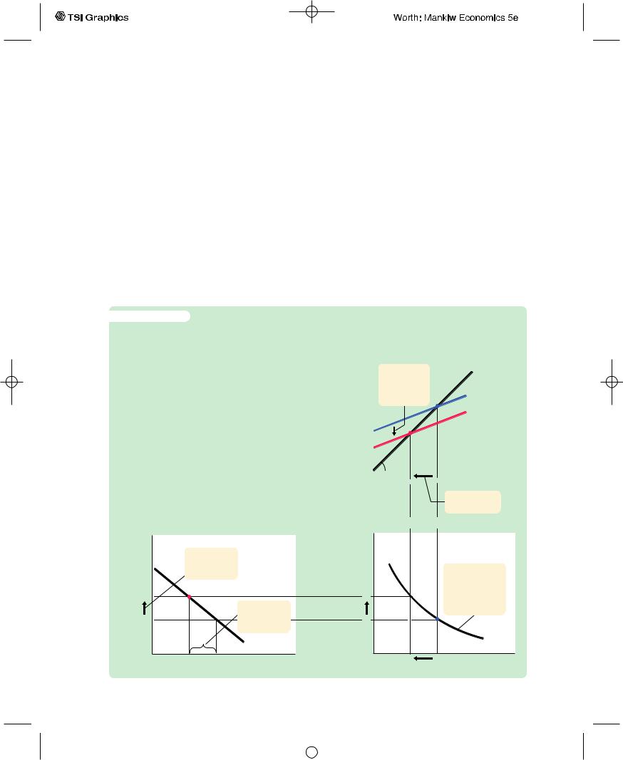
The Keynesian cross is only a steppingstone on our path to the IS–LM model. The Keynesian cross is useful because it shows how the spending plans of households, firms, and the government determine the economy’s income. Yet it makes the simplifying assumption that the level of planned investment I is fixed. As we discussed in Chapter 3, an important macroeconomic relationship is that planned investment depends on the interest rate r.

To add this relationship between the interest rate and investment to our model, we write the level of planned investment as

I = I(r).

This investment function is graphed in panel (a) of Figure 10-7. Because the interest rate is the cost of borrowing to finance investment projects, an increase in

268 | P A R T I V Business Cycle Theory: The Economy in the Short Run

the interest rate reduces planned investment. As a result, the investment function slopes downward.

To determine how income changes when the interest rate changes, we can combine the investment function with the Keynesian-cross diagram. Because investment is inversely related to the interest rate, an increase in the interest rate from r1 to r2 reduces the quantity of investment from I(r1) to I(r2).The reduction in planned investment, in turn, shifts the planned-expenditure function downward, as in panel (b) of Figure 10-7.The shift in the planned-expenditure function causes the level of income to fall from Y1 to Y2. Hence, an increase in the interest rate lowers income.

The IS curve, shown in panel (c) of Figure 10-7, summarizes this relationship between the interest rate and the level of income. In essence, the IS curve combines the interaction between r and I expressed by the investment function and the interaction between I and Y demonstrated by the Keynesian cross. Because an increase in the interest rate causes planned investment to fall, which in turn causes income to fall, the IS curve slopes downward.

How Fiscal Policy Shifts the IS Curve

The IS curve shows us, for any given interest rate, the level of income that brings the goods market into equilibrium. As we learned from the Keynesian cross, the level of income also depends on fiscal policy.The IS curve is drawn for a given fiscal policy; that is, when we construct the IS curve, we hold G and T fixed. When fiscal policy changes, the IS curve shifts.

Figure 10-8 uses the Keynesian cross to show how an increase in government

purchases by DG shifts the IS curve.This figure is drawn for a given interest rate

−

r and thus for a given level of planned investment. The Keynesian cross shows that this change in fiscal policy raises planned expenditure and thereby increases equilibrium income from Y1 to Y2. Therefore, an increase in government purchases shifts the IS curve outward.

We can use the Keynesian cross to see how other changes in fiscal policy shift the IS curve. Because a decrease in taxes also expands expenditure and income, it too shifts the IS curve outward. A decrease in government purchases or an increase in taxes reduces income; therefore, such a change in fiscal policy shifts the IS curve inward.

In summary, the IS curve shows the combinations of the interest rate and the level of income that are consistent with equilibrium in the market for goods and services.The IS curve is drawn for a given fiscal policy. Changes in fiscal policy that raise the demand for goods and services shift the IS curve to the right. Changes in fiscal policy that reduce the demand for goods and services shift the IS curve to the left.

A Loanable-Funds Interpretation of the IS Curve

When we first studied the market for goods and services in Chapter 3, we noted an equivalence between the supply and demand for goods and services and the supply and demand for loanable funds.This equivalence provides another way to interpret the IS curve.