

Mankiw Macroeconomics (5th ed)
.pdfC H A P T E R 1 0 Aggregate Demand I | 269
f i g u r e 1 0 - 8
(a) The Keynesian Cross
Expenditure, E |
1. An increase in government |
Actual |
|
|
|||
|
purchases shifts planned |
expenditure |
|
|
expenditure upward by G, . . . |
Planned |
|
Y2 |
|
|
|
|
|
expenditure |
|
|
|
|
|
Y1
2. . . . which raises income
by G . . .
1 MPC
An Increase in Government Purchases Shifts the IS Curve Outward Panel (a) shows that an increase in government purchases raises planned expenditure. For any given interest rate, the upward shift in planned expenditure of DG leads to an increase in income
Y of DG/(1 − MPC). Therefore, in panel (b), the IS curve shifts to the right by this amount.
Y1 |
Y2 |
Income, output, Y |
(b) The IS Curve
Interest rate, r
r
3. . . . and shifts |
|
the IS curve to |
|
the right |
|
by |
G . |
1 |
MPC |
|
IS2 |
|
IS1 |
Y1 |
Y2 |
Income, output, Y |
Recall that the national income accounts identity can be written as
Y − C − G = I
S = I.
The left-hand side of this equation is national saving S, and the right-hand side is investment I. National saving represents the supply of loanable funds, and investment represents the demand for these funds.
User JOEWA:Job EFF01426:6264_ch10:Pg 269:27278#/eps at 100% *27278* |
Wed, Feb 13, 2002 10:17 AM |
|||
|
|
|
|
|
|
|
|
|
|
270 | P A R T I V Business Cycle Theory: The Economy in the Short Run
To see how the market for loanable funds produces the IS curve, substitute the consumption function for C and the investment function for I:
Y − C(Y − T ) − G = I(r).
The left-hand side of this equation shows that the supply of loanable funds depends on income and fiscal policy. The right-hand side shows that the demand for loanable funds depends on the interest rate.The interest rate adjusts to equilibrate the supply and demand for loans.
As Figure 10-9 illustrates, we can interpret the IS curve as showing the interest rate that equilibrates the market for loanable funds for any given level of income. When income rises from Y1 to Y2, national saving, which equals Y − C − G, increases. (Consumption rises by less than income, because the marginal propensity to consume is less than 1.) As panel (a) shows, the increased supply of loanable funds drives down the interest rate from r1 to r2.The IS curve in panel
(b) summarizes this relationship: higher income implies higher saving, which in turn implies a lower equilibrium interest rate. For this reason, the IS curve slopes downward.
This alternative interpretation of the IS curve also explains why a change in fiscal policy shifts the IS curve. An increase in government purchases or a decrease in taxes reduces national saving for any given level of income.The reduced supply of loanable funds raises the interest rate that equilibrates the market. Because the interest rate is now higher for any given level of income, the IS curve shifts upward in response to the expansionary change in fiscal policy.
Finally, note that the IS curve does not determine either income Y or the interest rate r. Instead, the IS curve is a relationship between Y and r arising in the
f i g u r e 1 0 - 9
(a) The Market for Loanable Funds
Interest rate, r
r1
r2
2. . . . causing the interest rate to drop.
1. An increase in income raises saving, . ..
I(r)
Investment,
Saving, I, S
(b) The IS Curve
Interest
rate, r 3. The IS curve summarizes these changes.
r1
r2
|
|
IS |
|
|
|
Y1 |
Y2 |
Income, |
|
|
output, Y |
A Loanable-Funds Interpretation of the IS Curve Panel (a) shows that an increase in income from Y1 to Y2 raises saving and thus lowers the interest rate that equilibrates the supply and demand for loanable funds. The IS curve in panel (b) expresses this negative relationship between income and the interest rate.
User JOEWA:Job EFF01426:6264_ch10:Pg 270:27279#/eps at 100% *27279* |
Wed, Feb 13, 2002 10:17 AM |
|||
|
|
|
|
|
|
|
|
|
|

C H A P T E R 1 0 Aggregate Demand I | 271
market for goods and services or, equivalently, the market for loanable funds.To determine the equilibrium of the economy, we need another relationship between these two variables, to which we now turn.
10-2 The Money Market and the LM Curve
The LM curve plots the relationship between the interest rate and the level of income that arises in the market for money balances.To understand this relationship, we begin by looking at a theory of the interest rate, called the theory of liquidity preference.
The Theory of Liquidity Preference
In his classic work The General Theory, Keynes offered his view of how the interest rate is determined in the short run.That explanation is called the theory of liquidity preference, because it posits that the interest rate adjusts to balance the supply and demand for the economy’s most liquid asset—money. Just as the Keynesian cross is a building block for the IS curve, the theory of liquidity preference is a building block for the LM curve.
To develop this theory, we begin with the supply of real money balances. If M stands for the supply of money and P stands for the price level, then M/P is the supply of real money balances.The theory of liquidity preference assumes there is a fixed supply of real money balances.That is,
s = − −
(M/P) M /P .
The money supply M is an exogenous policy variable chosen by a central bank, such as the Federal Reserve. The price level P is also an exogenous variable in this model. (We take the price level as given because the IS–LM model—our ultimate goal in this chapter—explains the short run when the price level is fixed.) These assumptions imply that the supply of real money balances is fixed and, in particular, does not depend on the interest rate.Thus, when we plot the supply of real money balances against the interest rate in Figure 10-10, we obtain a vertical supply curve.
Next, consider the demand for real money balances.The theory of liquidity preference posits that the interest rate is one determinant of how much money people choose to hold.The reason is that the interest rate is the opportunity cost of holding money: it is what you forgo by holding some of your assets as money, which does not bear interest, instead of as interest-bearing bank deposits or bonds. When the interest rate rises, people want to hold less of their wealth in the form of money. We can write the demand for real money balances as
(M/P)d = L(r),
User JOEWA:Job EFF01426:6264_ch10:Pg 271:27280#/eps at 100% *27280* |
Wed, Feb 13, 2002 10:17 AM |
|||
|
|
|
|
|
|
|
|
|
|
272 | P A R T I V Business Cycle Theory: The Economy in the Short Run
f i g u r e 1 0 - 1 0
Interest rate, r
Equilibrium interest rate
Demand, L (r)
M/P Real money balances, M/P
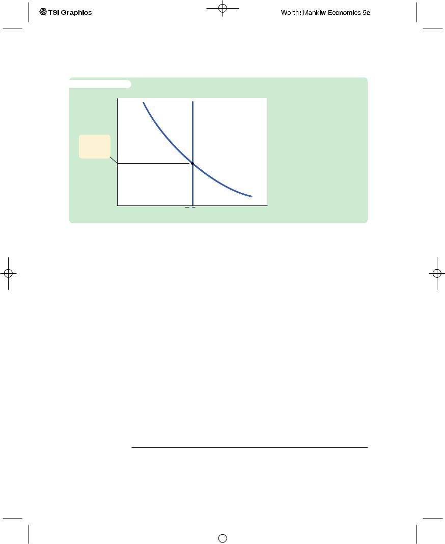
The Theory of Liquidity Preference The supply and demand for real money balances determine the interest rate. The supply curve for real money balances is vertical because the supply does not depend on the interest rate. The demand curve is downward sloping because a higher interest rate raises the cost of holding money and thus lowers the quantity demanded. At the equilibrium interest rate, the quantity of real money balances demanded equals the quantity supplied.
where the function L( ) shows that the quantity of money demanded depends on the interest rate.Thus, the demand curve in Figure 10-10 slopes downward because higher interest rates reduce the quantity of real money balances demanded.6
According to the theory of liquidity preference, the supply and demand for real money balances determine what interest rate prevails in the economy. That is, the interest rate adjusts to equilibrate the money market. As the figure shows, at the equilibrium interest rate, the quantity of real money balances demanded equals the quantity supplied.
How does the interest rate get to this equilibrium of money supply and money demand? The adjustment occurs because whenever the money market is not in equilibrium, people try to adjust their portfolios of assets and, in the process, alter the interest rate. For instance, if the interest rate is above the equilibrium level, the quantity of real money balances supplied exceeds the quantity demanded. Individuals holding the excess supply of money try to convert some of their non-interest-bearing money into interest-bearing bank deposits or bonds. Banks and bond issuers, who prefer to pay lower interest rates, respond to this excess supply of money by lowering the interest rates they offer. Conversely, if the interest rate is below the equilibrium level, so that the quantity of money demanded exceeds the quantity supplied, individuals try to obtain money by selling bonds or making bank withdrawals.To attract now-scarcer funds, banks and bond issuers respond by increasing the interest rates they offer. Eventually, the
6 Note that r is being used to denote the interest rate here, as it was in our discussion of the IS curve. More accurately, it is the nominal interest rate that determines money demand and the real interest rate that determines investment.To keep things simple, we are ignoring expected inflation, which creates the difference between the real and nominal interest rates.The role of expected inflation in the IS–LM model is explored in Chapter 11.
User JOEWA:Job EFF01426:6264_ch10:Pg 272:27281#/eps at 100% *27281* |
Wed, Feb 13, 2002 10:17 AM |
|||
|
|
|
|
|
|
|
|
|
|
C H A P T E R 1 0 Aggregate Demand I | 273
f i g u r e 1 0 - 1 1
Interest rate, r
1. A fall in the money supply. . .
r2
2. . . . raises r1 the interest
rate.
M2/P M1/P Real money balances, M/P
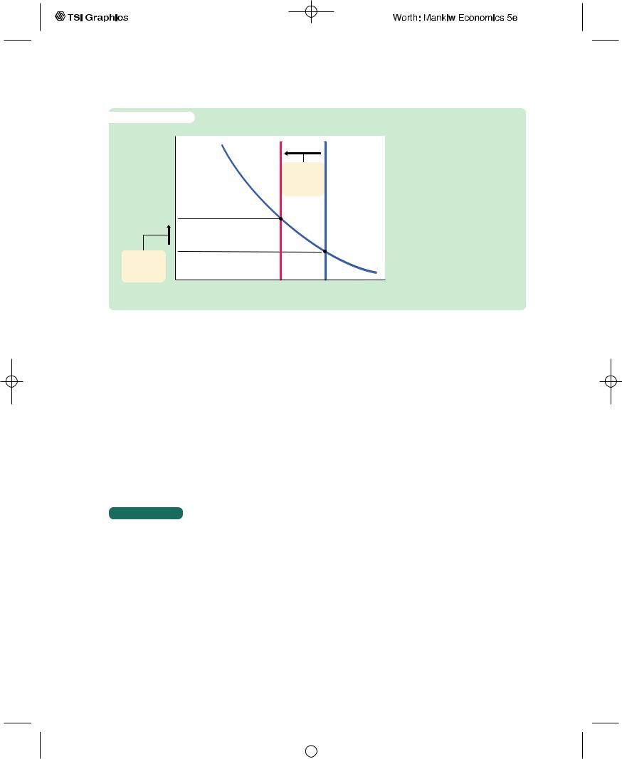
A Reduction in the Money Supply in the Theory of Liquidity Preference If the price level is fixed, a reduction in the money supply from M1 to M2 reduces the supply of real money balances. The equilibrium interest rate therefore rises from r1 to r2.
interest rate reaches the equilibrium level, at which people are content with their portfolios of monetary and nonmonetary assets.
Now that we have seen how the interest rate is determined, we can use the theory of liquidity preference to show how the interest rate responds to changes in the supply of money. Suppose, for instance, that the Fed suddenly decreases the money supply. A fall in M reduces M/P, because P is fixed in the model. The supply of real money balances shifts to the left, as in Figure 10-11.The equilibrium interest rate rises from r1 to r2, and the higher interest rate makes people satisfied to hold the smaller quantity of real money balances.The opposite would occur if the Fed had suddenly increased the money supply.Thus, according to the theory of liquidity preference, a decrease in the money supply raises the interest rate, and an increase in the money supply lowers the interest rate.
C A S E S T U D Y
Did Paul Volcker’s Monetary Tightening Raise or Lower Interest Rates?
The early 1980s saw the largest and quickest reduction in inflation in recent U.S. history. By the late 1970s inflation had reached the double-digit range; in 1979, consumer prices were rising at a rate of 11.3 percent per year. In October 1979, only two months after becoming the chairman of the Federal Reserve, Paul Volcker announced that monetary policy would aim to reduce the rate of inflation. This announcement began a period of tight money that, by 1983, brought the inflation rate down to about 3 percent.
How does such a monetary tightening influence interest rates? According to the theories we have been developing, the answer depends on the time horizon. Our analysis of the Fisher effect in Chapter 4 suggests that in the long run
User JOEWA:Job EFF01426:6264_ch10:Pg 273:27282#/eps at 100% *27282* |
Wed, Feb 13, 2002 10:17 AM |
|||
|
|
|
|
|
|
|
|
|
|

274 | P A R T I V Business Cycle Theory: The Economy in the Short Run
Volcker’s change in monetary policy would lower inflation, and this in turn would lead to lower nominal interest rates.Yet the theory of liquidity preference predicts that, in the short run when prices are sticky, anti-inflationary monetary policy would lead to falling real money balances and higher nominal interest rates.
Both conclusions are consistent with experience. Nominal interest rates did fall in the 1980s as inflation fell. But comparing the year before the October 1979 announcement and the year after, we find that real money balances (M1 divided by the CPI) fell 8.3 percent and the nominal interest rate (on short-term commercial loans) rose from 10.1 percent to 11.9 percent. Hence, although a monetary tightening leads to lower nominal interest rates in the long run, it leads to higher nominal interest rates in the short run.
Income, Money Demand, and the LM Curve
Having developed the theory of liquidity preference as an explanation for what determines the interest rate, we can now use the theory to derive the LM curve.We begin by considering the following question: How does a change in the economy’s level of income Y affect the market for real money balances? The answer (which should be familiar from Chapter 4) is that the level of income affects the demand for money.When income is high, expenditure is high, so people engage in more transactions that require the use of money.Thus, greater income implies greater money demand.We can express these ideas by writing the money demand function as
(M/P)d = L(r, Y ).
The quantity of real money balances demanded is negatively related to the interest rate and positively related to income.
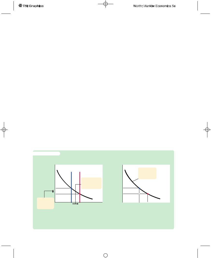
Using the theory of liquidity preference, we can figure out what happens to the equilibrium interest rate when the level of income changes. For example, consider what happens in Figure 10-12 when income increases from Y1 to Y2. As panel (a) illustrates, this increase in income shifts the money demand curve to the right. With the supply of real money balances unchanged, the interest rate must rise from r1 to r2 to equilibrate the money market.Therefore, according to the theory of liquidity preference, higher income leads to a higher interest rate.
The LM curve plots this relationship between the level of income and the interest rate.The higher the level of income, the higher the demand for real money balances, and the higher the equilibrium interest rate. For this reason, the LM curve slopes upward, as in panel (b) of Figure 10-12.
How Monetary Policy Shifts the LM Curve
The LM curve tells us the interest rate that equilibrates the money market at any level of income.Yet, as we saw earlier, the equilibrium interest rate also depends on the supply of real money balances, M/P. This means that the LM curve is
User JOEWA:Job EFF01426:6264_ch10:Pg 274:27283#/eps at 100% *27283* |
Wed, Feb 13, 2002 10:17 AM |
|||
|
|
|
|
|
|
|
|
|
|
f i g u r e 1 0 - 1 2
(a) The Market for Real Money Balances
Interest rate, r
r2
r1
2. . . .
increasing the interest rate.
1. An increase in income raises money demand, . . .
|
|
|
|
|
(r, Y2) |
|
|
|
|
|
L(r, Y1) |
|
|
|
|
|
|
|
|
|
|
|
Real money |
M/P |
|
||||
|
|
|
|
|
balances, M/P |
C H A P T E R 1 0 Aggregate Demand I | 275
(b) The LM Curve
Interest |
|
LM |
|
||
rate, r |
|
|
|||
|
|
|
|
||
|
|
|
|
|
|
|
r2 |
|
3. The LM curve |
|
|
|
|
|
|
||
|
|
|
summarizes |
|
|
|
r1 |
|
these changes in |
|
|
|
|
the money market |
|
||
|
|
|
equilibrium. |
|
|
|
|
|
|
|
|
|
|
Y1 |
Y2 Income, output, Y |
||
Deriving the LM Curve Panel (a) shows the market for real money balances: an increase in income from Y1 to Y2 raises the demand for money and thus raises the interest rate from r1 to r2. Panel (b) shows the LM curve summarizing this relationship between the interest rate and income: the higher the level of income, the higher the interest rate.
drawn for a given supply of real money balances. If real money balances change— for example, if the Fed alters the money supply—the LM curve shifts.
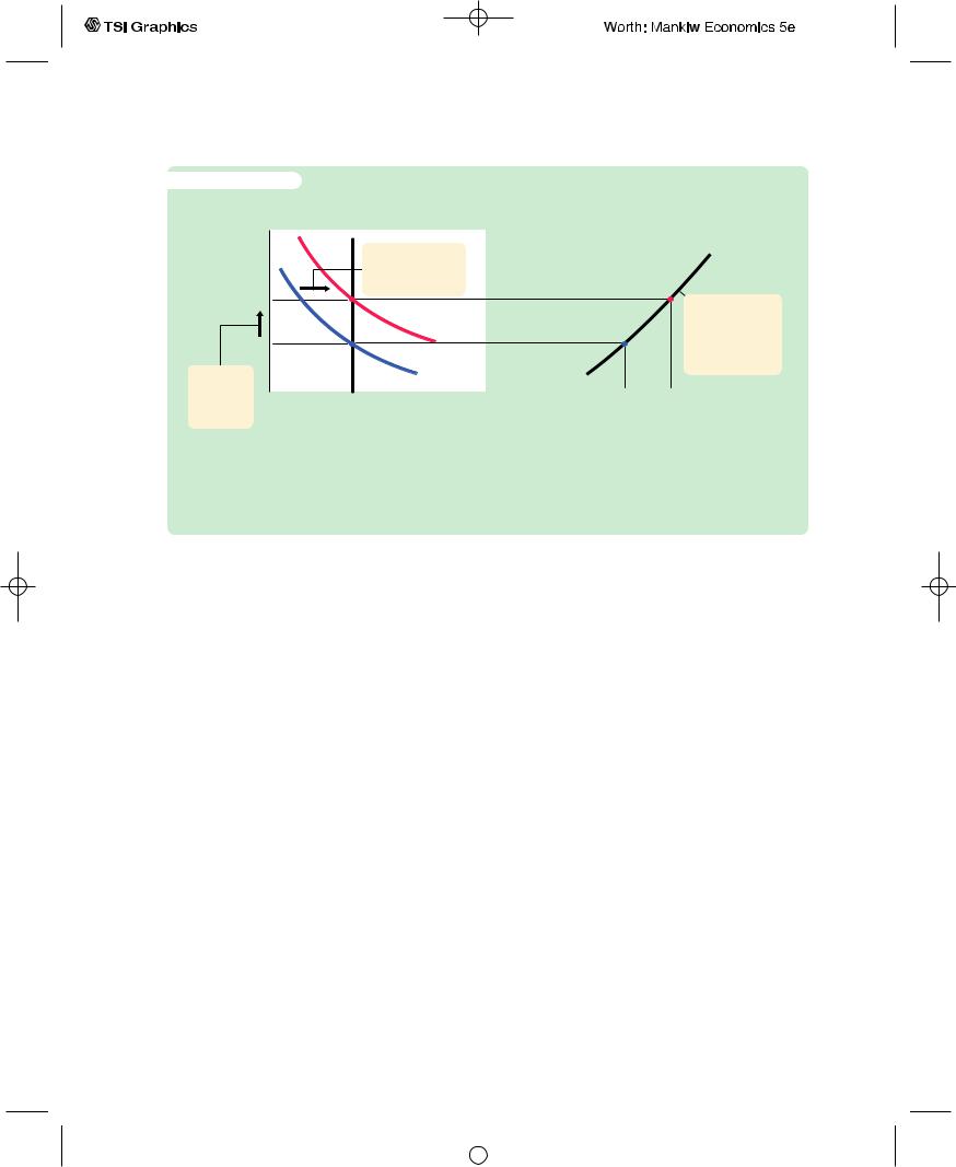
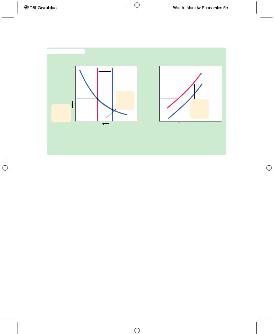
We can use the theory of liquidity preference to understand how monetary policy shifts the LM curve. Suppose that the Fed decreases the money supply from M1 to M2, which causes the supply of real money balances to fall from M1/P to M2/P. Figure 10-13 shows what happens. Holding constant the amount of income and thus the demand curve for real money balances, we see that a reduction in the supply of real money balances raises the interest rate that equilibrates the money market. Hence, a decrease in the money supply shifts the LM curve upward.
In summary, the LM curve shows the combinations of the interest rate and the level of income that are consistent with equilibrium in the market for real money balances.The LM curve is drawn for a given supply of real money balances. Decreases in the supply of real money balances shift the LM curve upward. Increases in the supply of real money balances shift the LM curve downward.
A Quantity-Equation Interpretation of the LM Curve
When we first discussed aggregate demand and the short-run determination of income in Chapter 9, we derived the aggregate demand curve from the quantity theory of money.We described the money market with the quantity equation,
MV = PY,
and assumed that velocity V is constant. This assumption implies that, for any given price level P, the supply of money M by itself determines the level of
User JOEWA:Job EFF01426:6264_ch10:Pg 275:27284#/eps at 100% *27284* |
Wed, Feb 13, 2002 10:17 AM |
|||
|
|
|
|
|
|
|
|
|
|
276 | P A R T I V Business Cycle Theory: The Economy in the Short Run
f i g u r e 1 0 - 1 3 |
|
(a) The Market for Real Money Balances |
(b) The LM Curve |
Interest rate, r |
|
Interest |
LM2 |
|
|
|
|
rate, r |
|
|
|
|
|
LM1 |
|
r2 |
1. The Fed |
r2 |
|
|
reduces |
3. . . . and |
||
|
|
the money |
|
|
2. . . . |
r1 |
supply, . . . |
r1 |
shifting the |
raising |
|
LM curve |
||
the interest |
|
L(r, Y) |
|
upward. |
rate . . . |
|
|
|
|
|
|
|
|
|
|
M2/P |
M1/P Real money |
Y |
Income, output, Y |
|
|
balances, |
|
|
|
|
M/P |
|
|
A Reduction in the Money Supply Shifts the LM Curve Upward Panel (a) shows that for
−
any given level of income Y, a reduction in the money supply raises the interest rate that equilibrates the money market. Therefore, the LM curve in panel (b) shifts upward.
income Y. Because the level of income does not depend on the interest rate, the quantity theory is equivalent to a vertical LM curve.
We can derive the more realistic upward-sloping LM curve from the quantity equation by relaxing the assumption that velocity is constant.The assumption of constant velocity is based on the assumption that the demand for real money balances depends only on the level of income. Yet, as we have noted in our discussion of the liquidity-preference model, the demand for real money balances also depends on the interest rate: a higher interest rate raises the cost of holding money and reduces money demand. When people respond to a higher interest rate by holding less money, each dollar they do hold must be used more often to support a given volume of transactions—that is, the velocity of money must increase.We can write this as
MV(r) = PY.
The velocity function V(r) indicates that velocity is positively related to the interest rate.
This form of the quantity equation yields an LM curve that slopes upward. Because an increase in the interest rate raises the velocity of money, it raises the level of income for any given money supply and price level. The LM curve expresses this positive relationship between the interest rate and income.
This equation also shows why changes in the money supply shift the LM curve. For any given interest rate and price level, the money supply and the level of income must move together. Thus, increases in the money supply shift the LM curve to the right, and decreases in the money supply shift the LM curve to the left.
User JOEWA:Job EFF01426:6264_ch10:Pg 276:27285#/eps at 100% *27285* |
Wed, Feb 13, 2002 10:17 AM |
|||
|
|
|
|
|
|
|
|
|
|
C H A P T E R 1 0 Aggregate Demand I | 277
Keep in mind that the quantity equation is merely another way to express the theory behind the LM curve. This quantity-theory interpretation of the LM curve is substantively the same as that provided by the theory of liquidity preference. In both cases, the LM curve represents a positive relationship between income and the interest rate that arises from the money market.
Finally, remember that the LM curve by itself does not determine either income Y or the interest rate r that will prevail in the economy. Like the IS curve, the LM curve is only a relationship between these two endogenous variables.The IS and LM curves together determine the economy’s equilibrium.
10-3 Conclusion: The Short-Run Equilibrium
We now have all the pieces of the IS–LM model. The two equations of this model are
Y = C(Y − T ) + I(r) + G |
IS, |
M/P = L(r, Y ) |
LM. |
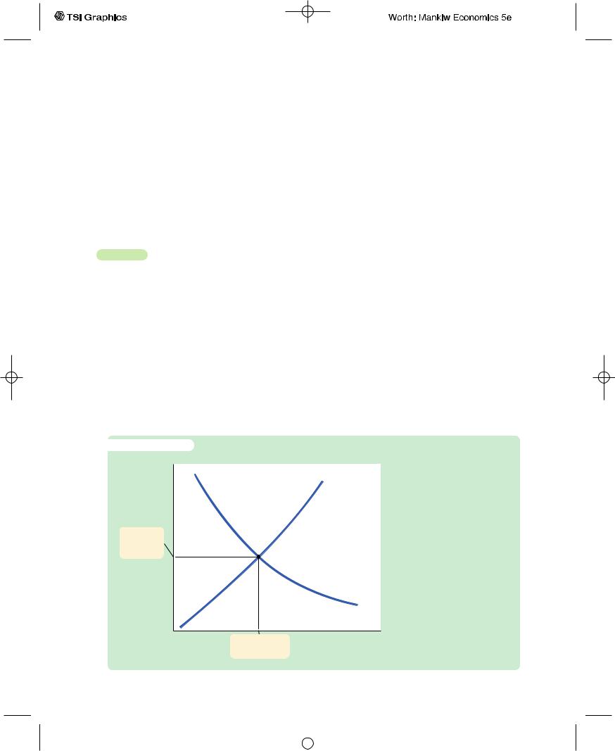
The model takes fiscal policy, G and T, monetary policy M, and the price level P as exogenous. Given these exogenous variables, the IS curve provides the combinations of r and Y that satisfy the equation representing the goods market, and the LM curve provides the combinations of r and Y that satisfy the equation representing the money market.These two curves are shown together in Figure 10-14.
f i g u r e 1 0 - 1 4
Interest rate, r
LM
Equilibrium interest rate
IS
Equilibrium in the IS–LM Model
The intersection of the IS and LM curves represents simultaneous equilibrium in the market for goods and services and in the market for real money balances for given values of government spending, taxes, the money supply, and the price level.
Equilibrium level |
Income, output, Y |
|
|
of income |
|
User JOEWA:Job EFF01426:6264_ch10:Pg 277:27286#/eps at 100% *27286* |
Wed, Feb 13, 2002 10:17 AM |
|||
|
|
|
|
|
|
|
|
|
|
278 | P A R T I V Business Cycle Theory: The Economy in the Short Run
The equilibrium of the economy is the point at which the IS curve and the LM curve cross.This point gives the interest rate r and the level of income Y that satisfy conditions for equilibrium in both the goods market and the money market. In other words, at this intersection, actual expenditure equals planned expenditure, and the demand for real money balances equals the supply.
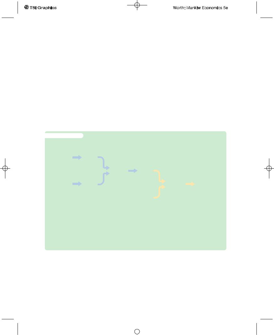
As we conclude this chapter, let’s recall that our ultimate goal in developing the IS–LM model is to analyze short-run fluctuations in economic activity. Figure 10-15 illustrates how the different pieces of our theory fit together. In this chapter we developed the Keynesian cross and the theory of liquidity preference as building blocks for the IS–LM model. As we see more fully in the next chapter, the IS–LM model helps explain the position and slope of the aggregate demand curve. The aggregate demand curve, in turn, is a piece of the model of aggregate supply and aggregate demand, which economists use to explain the short-run effects of policy changes and other events on national income.
f i g u r e 1 0 - 1 5
|
|
|
|
|
|
|
|
|
|
|
|
|
|
Keynesian |
|
IS Curve |
|
|
|
|
|
|
|
|
|
|
Cross |
|
|
|
|
|
|
|
|
|
||
|
|
|
|
|
|
|
|
|
|
|
|
|
|
|
|
|
|
IS–LM |
|
Aggregate |
|
|
|
|
|
|
|
|
|
|
|
|
|
|
||||
|
|
|
|
|
|
Demand |
|
|
|
|
|
|
|
|
|
|
|
Model |
|
|
|
|
|
|
|
|
|
|
|
|
|
Curve |
|
Model of |
|
Explanation |
|
|
|
|
|
|
|
|
|
|
|
||||
|
|
|
|
|
|
|
|
|
|
|||
|
Theory of |
|
|
|
|
|
|
|
Aggregate |
|
|
|
|
|
|
|
|
|
|
|
|
of Short-Run |
|
||
|
Liquidity |
|
LM Curve |
|
|
|
|
|
Supply and |
|
|
|
|
|
|
|
|
|
|
Economic |
|
||||
|
Preference |
|
|
|
|
|
|
|
Aggregate |
|
|
|
|
|
|
|
|
|
|
|
|
Fluctuations |
|
||
|
|
|
|
|
|
|
Aggregate |
|
Demand |
|
|
|
|
|
|
|
|
|
|
|
|
|
|
||
|
|
|
|
|
|
|
|
|
|
|
|
|
|
|
|
|
|
|
|
Supply |
|
|
|
|
|
|
|
|
|
|
|
|
Curve |
|
|
|
|
|
|
|
|
|
|
|
|
|
|
|
|
|
|
|
|
|
|
|
|
|
|
|
|
|
|
|
The Theory of Short-Run Fluctuations This schematic diagram shows how the different pieces of the theory of short-run fluctuations fit together. The Keynesian cross explains the IS curve, and the theory of liquidity preference explains the LM curve. The IS and LM curves together yield the IS–LM model, which explains the aggregate demand curve. The aggregate demand curve is part of the model of aggregate supply and aggregate demand, which economists use to explain short-run fluctuations in economic activity.
Summary
1.The Keynesian cross is a basic model of income determination. It takes fiscal policy and planned investment as exogenous and then shows that there is one level of national income at which actual expenditure equals planned expenditure. It shows that changes in fiscal policy have a multiplied impact on income.
User JOEWA:Job EFF01426:6264_ch10:Pg 278:27287#/eps at 100% *27287* |
Wed, Feb 13, 2002 10:17 AM |
|||
|
|
|
|
|
|
|
|
|
|