Mankiw Macroeconomics (5th ed)

C H A P T E R 1 1 Aggregate Demand II | 289

Shocks to the LM curve arise from exogenous changes in the demand for money. For example, suppose that new restrictions on credit-card availability increase the amount of money people choose to hold. According to the theory of liquidity preference, when money demand rises, the interest rate necessary to equilibrate the money market is higher (for any given level of income and money supply). Hence, an increase in money demand shifts the LM curve upward, which tends to raise the interest rate and depress income.

In summary, several kinds of events can cause economic fluctuations by shifting the IS curve or the LM curve. Remember, however, that such fluctuations are not inevitable. Policymakers can try to use the tools of monetary and fiscal policy to offset exogenous shocks. If policymakers are sufficiently quick and skillful (admittedly, a big if ), shocks to the IS or LM curves need not lead to fluctuations in income or employment.

C A S E S T U D Y

The U.S. Slowdown of 2001

In 2001, the U.S. economy experienced a pronounced slowdown in economic activity.The unemployment rate rose from 3.9 percent in October 2000 to 4.9 percent in August 2001, and then to 5.8 percent in December 2001. In many ways, the slowdown looked like a typical recession driven by a fall in aggregate demand.

Two notable shocks can help explain this event.The first was a decline in the stock market. During the 1990s, the stock market experienced a boom of historic proportions, as investors became optimistic about the prospects of the new information technology. Some economists viewed the optimism as excessive at the time, and in hindsight this proved to be the case.When the optimism faded, average stock prices fell by about 25 percent from August 2000 to August 2001. The fall in the market reduced household wealth and thus consumer spending. In addition, the declining perceptions of the profitability of the new technologies led to a fall in investment spending. In the language of the IS–LM model, the IS curve shifted to the left.

The second shock was the terrorist attacks on New York and Washington on September 11, 2001. In the week after the attacks, the stock market fell another 12 percent, its biggest weekly loss since the Great Depression of the 1930s. Moreover, the attacks increased uncertainty about what the future would hold. Uncertainty can reduce spending because households and firms postpone some of their plans until the uncertainty is resolved. Thus, the terrorist attacks shifted the IS curve further to the left.

Fiscal and monetary policymakers were quick to respond to these events. Congress passed a tax cut in 2001, including an immediate tax rebate. One goal of the tax cut was to stimulate consumer spending. After the terrorist attacks, Congress increased government spending by appropriating funds to rebuild New York and to bail out the ailing airline industry. Both of these fiscal measures shifted the IS curve to the right.

290 | P A R T I V Business Cycle Theory: The Economy in the Short Run

At the same time, the Fed pursued expansionary monetary policy, shifting the LM curve to the right. Money growth accelerated, and interest rates fell.The interest rate on three-month Treasury bills fell from 6.4 percent in November of 2000 to 3.3 percent in August 2001, and then to 2.1 percent in September 2001 in the immediate aftermath of the terrorist attacks.

The magnitude of the slowdown of 2001 was not yet determined as this book was going to press. The big question was whether the policy measures undertaken were sufficient to offset the shocks that the economy had suffered. By the time you are reading this, you may know the answer.

What Is the Fed’s Policy Instrument—The Money Supply or the Interest Rate?

Our analysis of monetary policy has been based on the assumption that the Fed influences the economy by controlling the money supply. By contrast, when the media report on changes in Fed policy, they often simply say that the Fed has raised or lowered interest rates. Which is right? Even though these two views may seem different, both are correct, and it is important to understand why.

In recent years, the Fed has used the federal funds rate—the interest rate that banks charge one another for overnight loans—as its short-term policy instrument.When the Federal Open Market Committee meets every six weeks to set monetary policy, it votes on a target for this interest rate that will apply until the next meeting.After the meeting is over, the Fed’s bond traders in New York are told to conduct the open-market operations necessary to hit that target.These open-market operations change the money supply and shift the LM curve so that the equilibrium interest rate (determined by the intersection of the IS and LM curves) equals the target interest rate that the Federal Open Market Committee has chosen.

As a result of this operating procedure, Fed policy is often discussed in terms of changing interest rates. Keep in mind, however, that behind these changes in interest rates are the necessary changes in the money supply. A newspaper might report, for instance, that “the Fed has lowered interest rates.” To be more precise, we can translate this statement as meaning “the Federal Open Market Committee has instructed the Fed bond traders to buy bonds in open-market operations so as to increase the money supply, shift the LM curve, and reduce the equilibrium interest rate to hit a new lower target.”

Why has the Fed chosen to use an interest rate, rather than the money supply, as its short-term policy instrument? One possible answer is that shocks to the LM curve are more prevalent than shocks to the IS curve.When the Fed targets interest rates, it automatically offsets LM shocks by altering the money supply, but the policy exacerbates IS shocks. If LM shocks are the more prevalent type, then a policy of targeting the interest rate leads to greater economic stability than a policy of targeting the money supply. (Problem 7 at the end of this chapter asks you to analyze this issue more fully.)

Another possible reason for using the interest rate as the short-term policy instrument is that interest rates are easier to measure than the money supply.As we

C H A P T E R 1 1 Aggregate Demand II | 291

saw in Chapter 4, the Fed has several different measures of money—M1, M2, and so on—which sometimes move in different directions. Rather than deciding which measure is best, the Fed avoids the question by using the federal funds rate as its policy instrument.

11-2 IS–LM as a Theory of Aggregate Demand

We have been using the IS–LM model to explain national income in the short run when the price level is fixed. To see how the IS–LM model fits into the model of aggregate supply and aggregate demand introduced in Chapter 9, we now examine what happens in the IS–LM model if the price level is allowed to change. As was promised when we began our study of this model, the IS–LM model provides a theory to explain the position and slope of the aggregate demand curve.

From the IS–LM Model to the Aggregate Demand Curve

Recall from Chapter 9 that the aggregate demand curve describes a relationship between the price level and the level of national income. In Chapter 9 this relationship was derived from the quantity theory of money.The analysis showed that for a given money supply, a higher price level implies a lower level of income. Increases in the money supply shift the aggregate demand curve to the right, and decreases in the money supply shift the aggregate demand curve to the left.

To understand the determinants of aggregate demand more fully, we now use the IS–LM model, rather than the quantity theory, to derive the aggregate demand curve. First, we use the IS–LM model to show why national income falls as the price level rises—that is, why the aggregate demand curve is downward sloping. Second, we examine what causes the aggregate demand curve to shift.

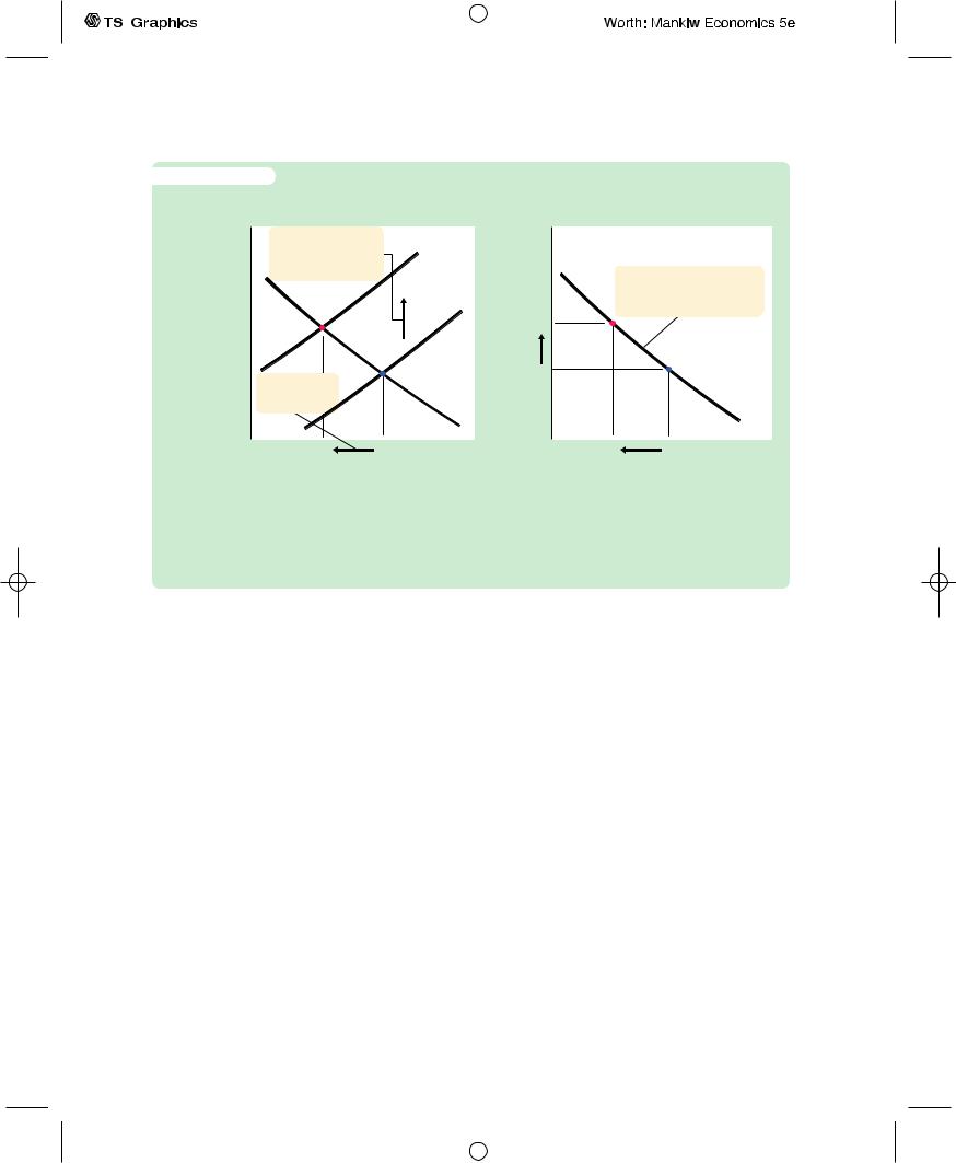
To explain why the aggregate demand curve slopes downward, we examine what happens in the IS–LM model when the price level changes.This is done in Figure 11-5. For any given money supply M, a higher price level P reduces the supply of real money balances M/P.A lower supply of real money balances shifts the LM curve upward, which raises the equilibrium interest rate and lowers the equilibrium level of income, as shown in panel (a). Here the price level rises from P1 to P2, and income falls from Y1 to Y2.The aggregate demand curve in panel

(b) plots this negative relationship between national income and the price level. In other words, the aggregate demand curve shows the set of equilibrium points that arise in the IS–LM model as we vary the price level and see what happens to income.

What causes the aggregate demand curve to shift? Because the aggregate demand curve is merely a summary of results from the IS–LM model, events that shift the IS curve or the LM curve (for a given price level) cause the aggregate demand curve to shift. For instance, an increase in the money supply raises income in the IS–LM model for any given price level; it thus shifts the

P1

2. . . . lowering income Y.

Deriving the Aggregate Demand Curve With the IS–LM Model Panel (a) shows the

IS–LM model: an increase in the price level from P1 to P2 lowers real money balances and thus shifts the LM curve upward. The shift in the LM curve lowers income from Y1 to Y2. Panel (b) shows the aggregate demand curve summarizing this relationship between the price level and income: the higher the price level, the lower the level of income.

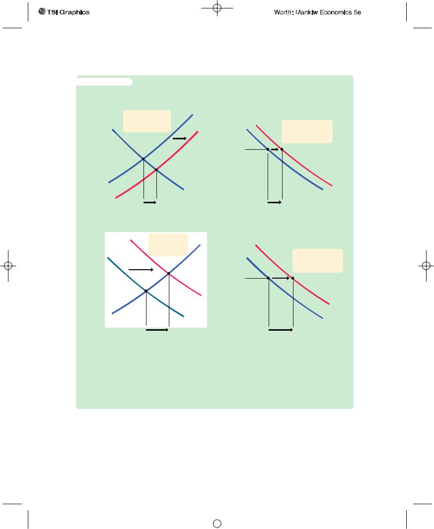
aggregate demand curve to the right, as shown in panel (a) of Figure 11-6. Similarly, an increase in government purchases or a decrease in taxes raises income in the IS-LM model for a given price level; it also shifts the aggregate demand curve to the right, as shown in panel (b) of Figure 11-6. Conversely, a decrease in the money supply, a decrease in government purchases, or an increase in taxes lowers income in the IS–LM model and shifts the aggregate demand curve to the left.

We can summarize these results as follows: A change in income in the IS–LM model resulting from a change in the price level represents a movement along the aggregate demand curve.A change in income in the IS–LM model for a fixed price level represents a shift in the aggregate demand curve.

The IS–LM Model in the Short Run and Long Run

The IS–LM model is designed to explain the economy in the short run when the price level is fixed.Yet, now that we have seen how a change in the price level influences the equilibrium in the IS–LM model, we can also use the model to describe the economy in the long run when the price level adjusts to ensure that the economy produces at its natural rate. By using the IS–LM model to describe the long run, we can show clearly how the Keynesian model of income determination differs from the classical model of Chapter 3.

C H A P T E R 1 1 Aggregate Demand II | 293

f i g u r e 1 1 - 6

How Monetary and Fiscal Policies Shift the Aggregate Demand Curve Panel (a) shows a monetary expansion. For any given price level, an increase in the money supply raises real money balances, shifts the LM curve downward, and raises income. Hence, an increase in the money supply shifts the aggregate demand curve to the right. Panel (b) shows a fiscal expansion, such as an increase in government purchases or a decrease in taxes. The fiscal expansion shifts the IS curve to the right and, for any given price level, raises income. Hence, a fiscal expansion shifts the aggregate demand curve to the right.

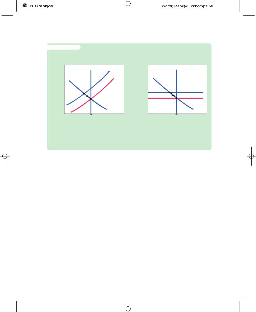
Panel (a) of Figure 11-7 shows the three curves that are necessary for under-

standing the short-run and long-run equilibria: the IS curve, the LM curve, and

−

the vertical line representing the natural rate of output Y . The LM curve is, as always, drawn for a fixed price level, P1.The short-run equilibrium of the economy is point K, where the IS curve crosses the LM curve. Notice that in this short-run equilibrium, the economy’s income is less than its natural rate.

The Short-Run and Long-Run Equilibria We can compare the short-run and long-run equilibria using either the IS–LM diagram in panel (a) or the aggregate supply– aggregate demand diagram in panel (b). In the short run, the price level is stuck at P1. The short-run equilibrium of the economy is therefore point K. In the long run, the price level adjusts so that the economy is at the natural rate. The long-run equilibrium is therefore point C.

Panel (b) of Figure 11-7 shows the same situation in the diagram of aggregate supply and aggregate demand. At the price level P1, the quantity of output demanded is below the natural rate. In other words, at the existing price level, there is insufficient demand for goods and services to keep the economy producing at its potential.

In these two diagrams we can examine the short-run equilibrium at which the economy finds itself and the long-run equilibrium toward which the economy gravitates. Point K describes the short-run equilibrium, because it assumes that the price level is stuck at P1. Eventually, the low demand for goods and services causes prices to fall, and the economy moves back toward its natural rate. When the price level reaches P2, the economy is at point C, the long-run equilibrium. The diagram of aggregate supply and aggregate demand shows that at point C, the quantity of goods and services demanded equals the natural rate of output.This long-run equilibrium is achieved in the IS–LM diagram by a shift in the LM curve: the fall in the price level raises real money balances and therefore shifts the LM curve to the right.

We can now see the key difference between Keynesian and classical approaches to the determination of national income. The Keynesian assumption (represented by point K) is that the price level is stuck. Depending on monetary policy, fiscal policy, and the other determinants of aggregate demand, output may deviate from the natural rate.The classical assumption (represented by point C) is that the price level is fully flexible.The price level adjusts to ensure that national income is always at the natural rate.

C H A P T E R 1 1 Aggregate Demand II | 295

To make the same point somewhat differently, we can think of the economy as being described by three equations.The first two are the IS and LM equations:

The IS equation describes the goods market, and the LM equation describes the money market. These two equations contain three endogenous variables: Y, P, and r.The Keynesian approach is to complete the model with the assumption of fixed prices, so the Keynesian third equation is

P = P1.

This assumption implies that r and Y must adjust to satisfy the IS and LM equations.The classical approach is to complete the model with the assumption that output reaches the natural rate, so the classical third equation is

= −

Y Y .

This assumption implies that r and P must adjust to satisfy the IS and LM equations.

Which assumption is most appropriate? The answer depends on the time horizon.The classical assumption best describes the long run. Hence, our longrun analysis of national income in Chapter 3 and prices in Chapter 4 assumes that output equals the natural rate.The Keynesian assumption best describes the short run.Therefore, our analysis of economic fluctuations relies on the assumption of a fixed price level.

11-3 The Great Depression

Now that we have developed the model of aggregate demand, let’s use it to address the question that originally motivated Keynes: What caused the Great Depression? Even today, more than half a century after the event, economists continue to debate the cause of this major economic downturn.The Great Depression provides an extended case study to show how economists use the IS–LM model to analyze economic fluctuations.1

Before turning to the explanations economists have proposed, look at Table 11-2, which presents some statistics regarding the Depression.These statistics are the battlefield on which debate about the Depression takes place. What do you think happened? An IS shift? An LM shift? Or something else?

1 For a flavor of the debate, see Milton Friedman and Anna J. Schwartz, A Monetary History of the United States, 1867–1960 (Princeton, NJ: Princeton University Press, 1963); Peter Temin, Did Monetary Forces Cause the Great Depression? (NewYork:W.W. Norton, 1976); the essays in Karl Brunner, ed., The Great Depression Revisited (Boston: Martinus Nijhoff, 1981); and the symposium on the Great Depression in the Spring 1993 issue of the Journal of Economic Perspectives.

296 | P A R T I V Business Cycle Theory: The Economy in the Short Run

t a b l e 1 1 - 2

What Happened During the Great Depression?

Source: Historical Statistics of the United States, Colonial Times to 1970, Parts I and II (Washington, DC: U.S. Department of Commerce, Bureau of Census, 1975).

Note: (1) The unemployment rate is series D9. (2) Real GNP, consumption, investment, and government purchases are series F3, F48, F52, and F66, and are measured in billions of 1958 dollars. (3) The interest rate is the prime Commercial

The Spending Hypothesis: Shocks to the IS Curve

Table 11-2 shows that the decline in income in the early 1930s coincided with falling interest rates.This fact has led some economists to suggest that the cause of the decline may have been a contractionary shift in the IS curve.This view is sometimes called the spending hypothesis, because it places primary blame for the Depression on an exogenous fall in spending on goods and services.

Economists have attempted to explain this decline in spending in several ways. Some argue that a downward shift in the consumption function caused the contractionary shift in the IS curve.The stock market crash of 1929 may have been partly responsible for this shift: by reducing wealth and increasing uncertainty about the future prospects of the U.S. economy, the crash may have induced consumers to save more of their income rather than spending it.

Others explain the decline in spending by pointing to the large drop in investment in housing. Some economists believe that the residential investment boom of the 1920s was excessive and that once this “overbuilding’’ became apparent, the demand for residential investment declined drastically. Another possible explanation for the fall in residential investment is the reduction in immigration in the 1930s: a more slowly growing population demands less new housing.

Once the Depression began, several events occurred that could have reduced spending further. First, many banks failed in the early 1930s, in part because of inadequate bank regulation, and these bank failures may have exacerbated the fall in investment spending. Banks play the crucial role of getting the funds available

C H A P T E R 1 1 Aggregate Demand II | 297

Paper rate, 4–6 months, series ×445. (4) The money supply is series ×414, currency plus demand deposits, measured in billions of dollars. (5) The price level is the GNP deflator (1958 = 100), series E1. (6) The inflation rate is the percentage change in the price level series. (7) Real money balances, calculated by dividing the money supply by the price level and multiplying by 100, are in billions of 1958 dollars.

for investment to those households and firms that can best use them.The closing of many banks in the early 1930s may have prevented some businesses from getting the funds they needed for capital investment and, therefore, may have led to a further contractionary shift in the investment function.2

In addition, the fiscal policy of the 1930s caused a contractionary shift in the IS curve. Politicians at that time were more concerned with balancing the budget than with using fiscal policy to keep production and employment at their natural rates. The Revenue Act of 1932 increased various taxes, especially those falling on lowerand middle-income consumers.3 The Democratic platform of that year expressed concern about the budget deficit and advocated an “immediate and drastic reduction of governmental expenditures.’’ In the midst of historically high unemployment, policymakers searched for ways to raise taxes and reduce government spending.

There are, therefore, several ways to explain a contractionary shift in the IS curve. Keep in mind that these different views may all be true.There may be no single explanation for the decline in spending. It is possible that all of these changes coincided and that together they led to a massive reduction in spending.

2Ben Bernanke, “Non-Monetary Effects of the Financial Crisis in the Propagation of the Great Depression,’’ American Economic Review 73 (June 1983): 257–276.

3E. Cary Brown,“Fiscal Policy in the ’Thirties:A Reappraisal,’’ American Economic Review 46 (December 1956): 857–879.

298 | P A R T I V Business Cycle Theory: The Economy in the Short Run

The Money Hypothesis: A Shock to the LM Curve

Table 11-2 shows that the money supply fell 25 percent from 1929 to 1933, during which time the unemployment rate rose from 3.2 percent to 25.2 percent. This fact provides the motivation and support for what is called the money hypothesis, which places primary blame for the Depression on the Federal Reserve for allowing the money supply to fall by such a large amount.4 The best-known advocates of this interpretation are Milton Friedman and Anna Schwartz, who defend it in their treatise on U.S. monetary history. Friedman and Schwartz argue that contractions in the money supply have caused most economic downturns and that the Great Depression is a particularly vivid example.

Using the IS–LM model, we might interpret the money hypothesis as explaining the Depression by a contractionary shift in the LM curve. Seen in this way, however, the money hypothesis runs into two problems.

The first problem is the behavior of real money balances. Monetary policy leads to a contractionary shift in the LM curve only if real money balances fall. Yet from 1929 to 1931 real money balances rose slightly, because the fall in the money supply was accompanied by an even greater fall in the price level. Although the monetary contraction may be responsible for the rise in unemployment from 1931 to 1933, when real money balances did fall, it cannot easily explain the initial downturn from 1929 to 1931.

The second problem for the money hypothesis is the behavior of interest rates. If a contractionary shift in the LM curve triggered the Depression, we should have observed higher interest rates.Yet nominal interest rates fell continuously from 1929 to 1933.

These two reasons appear sufficient to reject the view that the Depression was instigated by a contractionary shift in the LM curve. But was the fall in the money stock irrelevant? Next, we turn to another mechanism through which monetary policy might have been responsible for the severity of the Depres- sion—the deflation of the 1930s.

The Money Hypothesis Again: The Effects of

Falling Prices

From 1929 to 1933 the price level fell 25 percent. Many economists blame this deflation for the severity of the Great Depression.They argue that the deflation may have turned what in 1931 was a typical economic downturn into an unprecedented period of high unemployment and depressed income. If it is correct, this argument gives new life to the money hypothesis. Because the falling money supply was, plausibly, responsible for the falling price level, it could have been responsible for the severity of the Depression.To evaluate this argument, we must discuss how changes in the price level affect income in the IS–LM model.

4 We discuss the reasons for this large decrease in the money supply in Chapter 18, where we examine the money supply process in more detail. In particular, see the case study “Bank Failures and the Money Supply in the 1930s.”