Mankiw Macroeconomics (5th ed)

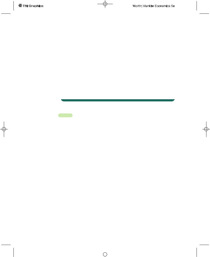
economy is in its long-run equilibrium, the short-run aggregate supply curve must cross this point as well.

Now suppose that the Fed reduces the money supply and the aggregate demand curve shifts downward, as in Figure 9-9. In the short run, prices are sticky, so the economy moves from point A to point B. Output and employment fall below their natural levels, which means the economy is in a recession. Over time, in response to the low demand, wages and prices fall. The gradual reduction in the price level moves the economy downward along the aggregate demand curve to point C, which is the new long-run equilibrium. In the new long-run equilibrium (point C), output and employment are back to their natural levels, but prices are lower than in the old long-run equilibrium (point A).Thus, a shift in aggregate demand affects output in the short run, but this effect dissipates over time as firms adjust their prices.

C A S E S T U D Y

Gold, Greenbacks, and the Contraction of the 1870s

The aftermath of the Civil War in the United States provides a vivid example of how contractionary monetary policy affects the economy. Before the war, the United States was on a gold standard. Paper dollars were readily convertible into gold. Under this policy, the quantity of gold determined the money supply and the price level.

In 1862, after the Civil War broke out, the Treasury announced that it would no longer redeem dollars for gold. In essence, this act replaced the gold standard with a system of fiat money. Over the next few years, the government printed large quantities of paper currency—called greenbacks for their color—and used

250 | P A R T I V Business Cycle Theory: The Economy in the Short Run

the seigniorage to finance wartime expenditure. Because of this increase in the money supply, the price level approximately doubled during the war.

When the war was over, much political debate centered on the question of whether to return to the gold standard. The Greenback party was formed with the primary goal of maintaining the system of fiat money. Eventually, however, the Greenback party lost the debate. Policymakers decided to retire the greenbacks over time in order to reinstate the gold standard at the rate of exchange between dollars and gold that had prevailed before the war.Their goal was to return the value of the dollar to its former level.

Returning to the gold standard in this way required reversing the wartime rise in prices, which meant aggregate demand had to fall. (To be more precise, the growth in aggregate demand needed to fall short of the growth in the natural rate of output.) As the price level fell, the economy experienced a recession from 1873 to 1879, the longest on record. By 1879, the price level was back to its level before the war, and the gold standard was reinstated.

9-4 Stabilization Policy

Fluctuations in the economy as a whole come from changes in aggregate supply or aggregate demand. Economists call exogenous changes in these curves shocks to the economy. A shock that shifts the aggregate demand curve is called a demand shock, and a shock that shifts the aggregate supply curve is called a supply shock.These shocks disrupt economic well-being by pushing output and employment away from their natural rates. One goal of the model of aggregate supply and aggregate demand is to show how shocks cause economic fluctuations.

Another goal of the model is to evaluate how macroeconomic policy can respond to these shocks. Economists use the term stabilization policy to refer to policy actions aimed at reducing the severity of short-run economic fluctuations. Because output and employment fluctuate around their long-run natural rates, stabilization policy dampens the business cycle by keeping output and employment as close to their natural rates as possible.

In the coming chapters, we examine in detail how stabilization policy works and what practical problems arise in its use. Here we begin our analysis of stabilization policy by examining how monetary policy might respond to shocks. Monetary policy is an important component of stabilization policy because, as we have seen, the money supply has a powerful impact on aggregate demand.

Shocks to Aggregate Demand

Consider an example of a demand shock: the introduction and expanded availability of credit cards. Because credit cards are often a more convenient way to make purchases than using cash, they reduce the quantity of money that people choose to hold.This reduction in money demand is equivalent to an increase in

C H A P T E R 9 Introduction to Economic Fluctuations | 251

the velocity of money.When each person holds less money, the money demand parameter k falls.This means that each dollar of money moves from hand to hand more quickly, so velocity V (= 1/k) rises.

If the money supply is held constant, the increase in velocity causes nominal spending to rise and the aggregate demand curve to shift outward, as in Figure 9-10. In the short run, the increase in demand raises the output of the economy— it causes an economic boom. At the old prices, firms now sell more output. Therefore, they hire more workers, ask their existing workers to work longer hours, and make greater use of their factories and equipment.

Over time, the high level of aggregate demand pulls up wages and prices. As the price level rises, the quantity of output demanded declines, and the economy gradually approaches the natural rate of production. But during the transition to the higher price level, the economy’s output is higher than the natural rate.

What can the Fed do to dampen this boom and keep output closer to the natural rate? The Fed might reduce the money supply to offset the increase in velocity. Offsetting the change in velocity would stabilize aggregate demand.Thus, the Fed can reduce or even eliminate the impact of demand shocks on output and employment if it can skillfully control the money supply.Whether the Fed in fact has the necessary skill is a more difficult question, which we take up in Chapter 14.

Shocks to Aggregate Supply

Shocks to aggregate supply, as well as shocks to aggregate demand, can cause economic fluctuations.A supply shock is a shock to the economy that alters the cost of producing goods and services and, as a result, the prices that firms charge.

252 | P A R T I V Business Cycle Theory: The Economy in the Short Run

Because supply shocks have a direct impact on the price level, they are sometimes called price shocks. Here are some examples:

A drought that destroys crops.The reduction in food supply pushes up food prices.

A new environmental protection law that requires firms to reduce their emissions of pollutants. Firms pass on the added costs to customers in the form of higher prices.

An increase in union aggressiveness.This pushes up wages and the prices of the goods produced by union workers.

The organization of an international oil cartel. By curtailing competition, the major oil producers can raise the world price of oil.

All these events are adverse supply shocks, which means they push costs and prices upward. A favorable supply shock, such as the breakup of an international oil cartel, reduces costs and prices.

Figure 9-11 shows how an adverse supply shock affects the economy. The short-run aggregate supply curve shifts upward. (The supply shock may also lower the natural level of output and thus shift the long-run aggregate supply curve to the left, but we ignore that effect here.) If aggregate demand is held constant, the economy moves from point A to point B: the price level rises and the amount of output falls below the natural rate. An experience like this is called stagflation, because it combines stagnation (falling output) with inflation (rising prices).

Faced with an adverse supply shock, a policymaker controlling aggregate demand, such as the Fed, has a difficult choice between two options. The first option, implicit in Figure 9-11, is to hold aggregate demand constant. In this case, output and employment are lower than the natural rate. Eventually, prices

C H A P T E R 9 Introduction to Economic Fluctuations | 253

will fall to restore full employment at the old price level (point A). But the cost of this adjustment process is a painful recession.

The second option, illustrated in Figure 9-12, is to expand aggregate demand to bring the economy toward the natural rate more quickly. If the increase in aggregate demand coincides with the shock to aggregate supply, the economy goes immediately from point A to point C. In this case, the Fed is said to accommodate the supply shock.The drawback of this option, of course, is that the price level is permanently higher.There is no way to adjust aggregate demand to maintain full employment and keep the price level stable.

C A S E S T U D Y

How OPEC Helped Cause Stagflation in the 1970s and Euphoria in the 1980s

The most disruptive supply shocks in recent history were caused by OPEC, the Organization of Petroleum Exporting Countries. In the early 1970s, OPEC’s coordinated reduction in the supply of oil nearly doubled the world price.This increase in oil prices caused stagflation in most industrial countries.These statistics show what happened in the United States:

254 | P A R T I V Business Cycle Theory: The Economy in the Short Run

The 68-percent increase in the price of oil in 1974 was an adverse supply shock of major proportions.As one would have expected, it led to both higher inflation and higher unemployment.

A few years later, when the world economy had nearly recovered from the first OPEC recession, almost the same thing happened again. OPEC raised oil prices, causing further stagflation. Here are the statistics for the United States:

The increases in oil prices in 1979, 1980, and 1981 again led to double-digit inflation and higher unemployment.

In the mid-1980s, political turmoil among the Arab countries weakened OPEC’s ability to restrain supplies of oil. Oil prices fell, reversing the stagflation of the 1970s and the early 1980s. Here’s what happened:

In 1986 oil prices fell by nearly half. This favorable supply shock led to one of the lowest inflation rates experienced in recent U.S. history and to falling unemployment.

More recently, OPEC has not been a major cause of economic fluctuations. This is in part because OPEC has been less successful at raising the price of oil. Although world oil prices have fluctuated, the changes have not been as large as those experienced during the 1970s, and the real price of oil has never returned to the peaks reached in the early 1980s. Moreover, conservation efforts and technological changes have made the economy less susceptible to oil shocks. The amount of oil consumed per unit of real GDP has fallen about 40 percent over the past three decades.

But we should not be too sanguine.The experiences of the 1970s and 1980s could always be repeated. Events in the Middle East are a potential source of shocks to economies around the world.3

3 Some economists have suggested that changes in oil prices played a major role in economic fluctuations even before the 1970s. See James D. Hamilton, “Oil and the Macroeconomy Since World War II,’’ Journal of Political Economy 91 (April 1983): 228–248.

C H A P T E R 9 Introduction to Economic Fluctuations | 255

9-5 Conclusion

This chapter introduced a framework to study economic fluctuations: the model of aggregate supply and aggregate demand.The model is built on the assumption that prices are sticky in the short run and flexible in the long run. It shows how shocks to the economy cause output to deviate temporarily from the level implied by the classical model.

The model also highlights the role of monetary policy. Poor monetary policy can be a source of shocks to the economy. A well-run monetary policy can respond to shocks and stabilize the economy.

In the chapters that follow, we refine our understanding of this model and our analysis of stabilization policy. Chapters 10 through 12 go beyond the quantity equation to refine our theory of aggregate demand.This refinement shows that aggregate demand depends on fiscal policy as well as monetary policy. Chapter 13 examines aggregate supply in more detail. Chapter 14 examines the debate over the virtues and limits of stabilization policy.

Summary

1.The crucial difference between the long run and the short run is that prices are flexible in the long run but sticky in the short run.The model of aggregate supply and aggregate demand provides a framework to analyze economic fluctuations and see how the impact of policies varies over different time horizons.

2.The aggregate demand curve slopes downward. It tells us that the lower the price level, the greater the aggregate quantity of goods and services demanded.

3.In the long run, the aggregate supply curve is vertical because output is determined by the amounts of capital and labor and by the available technology, but not by the level of prices.Therefore, shifts in aggregate demand affect the price level but not output or employment.

4.In the short run, the aggregate supply curve is horizontal, because wages and prices are sticky at predetermined levels. Therefore, shifts in aggregate demand affect output and employment.

5.Shocks to aggregate demand and aggregate supply cause economic fluctuations. Because the Fed can shift the aggregate demand curve, it can attempt to offset these shocks to maintain output and employment at their natural rates.

K E Y C O N C E P T S

256 | P A R T I V Business Cycle Theory: The Economy in the Short Run

Q U E S T I O N S F O R R E V I E W

P R O B L E M S A N D A P P L I C A T I O N S

C H A P T1E R 0 T E N

Aggregate Demand I

I shall argue that the postulates of the classical theory are applicable to a

special case only and not to the general case. . . . Moreover, the characteris-

tics of the special case assumed by the classical theory happen not to be

those of the economic society in which we actually live, with the result that

its teaching is misleading and disastrous if we attempt to apply it to the

facts of experience.

— John Maynard Keynes, The General Theory

Of all the economic fluctuations in world history, the one that stands out as particularly large, painful, and intellectually significant is the Great Depression of the 1930s. During this time, the United States and many other countries experienced massive unemployment and greatly reduced incomes. In the worst year, 1933, one-fourth of the U.S. labor force was unemployed, and real GDP was 30 percent below its 1929 level.

This devastating episode caused many economists to question the validity of classical economic theory—the theory we examined in Chapters 3 through 6. Classical theory seemed incapable of explaining the Depression. According to that theory, national income depends on factor supplies and the available technology, neither of which changed substantially from 1929 to 1933. After the onset of the Depression, many economists believed that a new model was needed to explain such a large and sudden economic downturn and to suggest government policies that might reduce the economic hardship so many people faced.

In 1936 the British economist John Maynard Keynes revolutionized economics with his book The General Theory of Employment, Interest, and Money. Keynes proposed a new way to analyze the economy, which he presented as an alternative to classical theory. His vision of how the economy works quickly became a center of controversy.Yet, as economists debated The General Theory, a new understanding of economic fluctuations gradually developed.

Keynes proposed that low aggregate demand is responsible for the low income and high unemployment that characterize economic downturns. He criticized classical theory for assuming that aggregate supply alone—capital, labor, and technol- ogy—determines national income. Economists today reconcile these two views

| 257

258 | P A R T I V Business Cycle Theory: The Economy in the Short Run

with the model of aggregate demand and aggregate supply introduced in Chapter 9. In the long run, prices are flexible, and aggregate supply determines income. But in the short run, prices are sticky, so changes in aggregate demand influence income.

In this chapter and the next, we continue our study of economic fluctuations by looking more closely at aggregate demand. Our goal is to identify the variables that shift the aggregate demand curve, causing fluctuations in national income. We also examine more fully the tools policymakers can use to influence aggregate demand. In Chapter 9 we derived the aggregate demand curve from the quantity theory of money, and we showed that monetary policy can shift the aggregate demand curve. In this chapter we see that the government can influence aggregate demand with both monetary and fiscal policy.

The model of aggregate demand developed in this chapter, called the IS–LM model, is the leading interpretation of Keynes’s theory.The goal of the model is to show what determines national income for any given price level. There are two ways to view this exercise.We can view the IS–LM model as showing what causes income to change in the short run when the price level is fixed. Or we can view the model as showing what causes the aggregate demand curve to shift. These two views of the model are equivalent: as Figure 10-1 shows, in the short run when the price level is fixed, shifts in the aggregate demand curve lead to changes in national income.

The two parts of the IS–LM model are, not surprisingly, the IS curve and the LM curve. IS stands for “investment’’ and “saving,’’ and the IS curve represents what’s going on in the market for goods and services (which we first discussed in Chapter 3). LM stands for “liquidity’’ and “money,’’ and the LM curve represents what’s happening to the supply and demand for money (which we first discussed in Chapter 4). Because the interest rate influences both investment and money