Mankiw Macroeconomics (5th ed)

C H A P T E R 1 6 Consumption | 439

FYIPresent Value, or Why a $1,000,000 Prize Is Worth Only $623,000

period (C1 = Y1 and C2 = Y2), so there is neither saving nor borrowing between the two periods. At point B, the consumer consumes nothing in the first period (C1 = 0) and saves all income, so second-period consumption C2 is (1 + r)Y1 + Y2. At point C, the consumer plans to consume nothing in the second period (C2 = 0) and borrows as much as possible against second-period income, so first-period

440 | P A R T V I More on the Microeconomics Behind Macroeconomics

consumption C1 is Y1 + Y2/(1 + r). Of course, these are only three of the many combinations of firstand second-period consumption that the consumer can afford: all the points on the line from B to C are available to the consumer.

Consumer Preferences

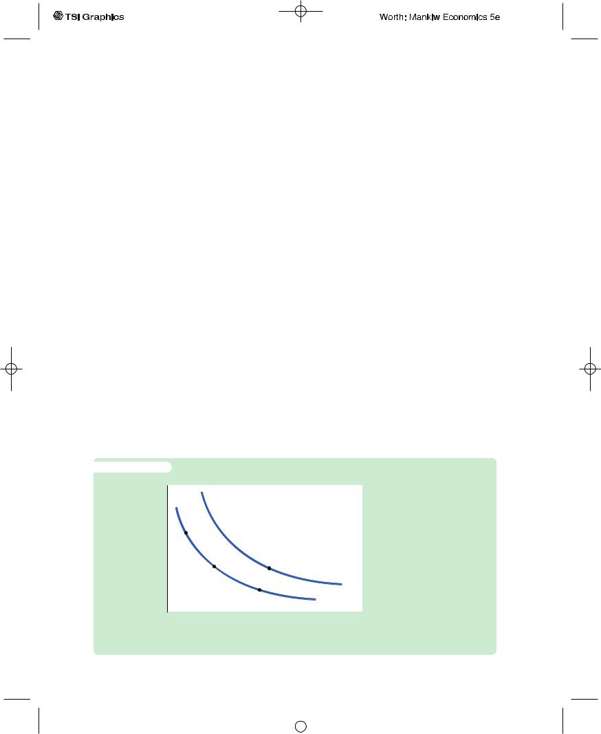
The consumer’s preferences regarding consumption in the two periods can be represented by indifference curves. An indifference curve shows the combinations of first-period and second-period consumption that make the consumer equally happy.

Figure 16-4 shows two of the consumer’s many indifference curves.The consumer is indifferent among combinations W, X, and Y, because they are all on the same curve. Not surprisingly, if the consumer’s first-period consumption is reduced, say from point W to point X, second-period consumption must increase to keep him equally happy. If first-period consumption is reduced again, from point X to point Y, the amount of extra second-period consumption he requires for compensation is greater.

The slope at any point on the indifference curve shows how much secondperiod consumption the consumer requires in order to be compensated for a 1-unit reduction in first-period consumption.This slope is the marginal rate of substitution between first-period consumption and second-period consumption. It tells us the rate at which the consumer is willing to substitute secondperiod consumption for first-period consumption.

Notice that the indifference curves in Figure 16-4 are not straight lines and, as a result, the marginal rate of substitution depends on the levels of consumption in the two periods. When first-period consumption is high and second-period consumption is low, as at point W, the marginal rate of substitution is low: the consumer requires only a little extra second-period consumption to give up

C H A P T E R 1 6 Consumption | 441

1 unit of first-period consumption. When first-period consumption is low and second-period consumption is high, as at point Y, the marginal rate of substitution is high: the consumer requires much additional second-period consumption to give up 1 unit of first-period consumption.

The consumer is equally happy at all points on a given indifference curve, but he prefers some indifference curves to others. Because he prefers more consumption to less, he prefers higher indifference curves to lower ones. In Figure 16-4, the consumer prefers the points on curve IC2 to the points on curve IC1.

The set of indifference curves gives a complete ranking of the consumer’s preferences. It tells us that the consumer prefers point Z to point W, but that may be obvious because point Z has more consumption in both periods.Yet compare point Z and point Y: point Z has more consumption in period one and less in period two. Which is preferred, Z or Y? Because Z is on a higher indifference curve than Y, we know that the consumer prefers point Z to point Y. Hence, we can use the set of indifference curves to rank any combinations of first-period and second-period consumption.

Optimization

Having discussed the consumer’s budget constraint and preferences, we can consider the decision about how much to consume. The consumer would like to end up with the best possible combination of consumption in the two periods— that is, on the highest possible indifference curve. But the budget constraint requires that the consumer also end up on or below the budget line, because the budget line measures the total resources available to him.

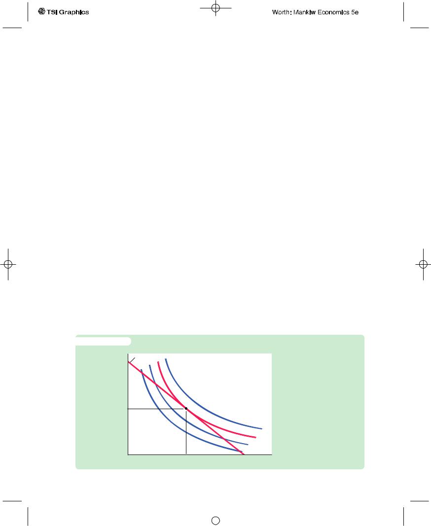
Figure 16-5 shows that many indifference curves cross the budget line. The highest indifference curve that the consumer can obtain without violating the budget constraint is the indifference curve that just barely touches the budget

442 | P A R T V I More on the Microeconomics Behind Macroeconomics

line, which is curve IC3 in the figure. The point at which the curve and line touch—point O for “optimum”—is the best combination of consumption in the two periods that the consumer can afford.

Notice that, at the optimum, the slope of the indifference curve equals the slope of the budget line.The indifference curve is tangent to the budget line.The slope of the indifference curve is the marginal rate of substitution MRS, and the slope of the budget line is 1 plus the real interest rate.We conclude that at point O,

MRS = 1 + r.

The consumer chooses consumption in the two periods so that the marginal rate of substitution equals 1 plus the real interest rate.

How Changes in Income Affect Consumption

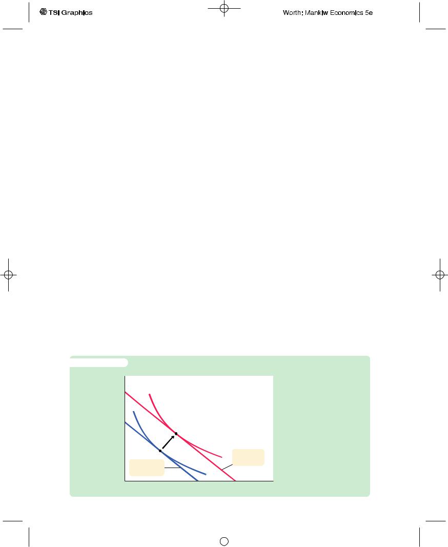
Now that we have seen how the consumer makes the consumption decision, let’s examine how consumption responds to an increase in income.An increase in either Y1 or Y2 shifts the budget constraint outward, as in Figure 16-6.The higher budget constraint allows the consumer to choose a better combination of firstand second-period consumption—that is, the consumer can now reach a higher indifference curve.

In Figure 16-6, the consumer responds to the shift in his budget constraint by choosing more consumption in both periods. Although it is not implied by the logic of the model alone, this situation is the most usual. If a consumer wants more of a good when his or her income rises, economists call it a normal good. The indifference curves in Figure 16-6 are drawn under the assumption that consumption in period one and consumption in period two are both normal goods.

The key conclusion from Figure 16-6 is that regardless of whether the increase in income occurs in the first period or the second period, the consumer spreads it over consumption in both periods. This behavior is sometimes called

C H A P T E R 1 6 Consumption | 443

consumption smoothing. Because the consumer can borrow and lend between periods, the timing of the income is irrelevant to how much is consumed today (except, of course, that future income is discounted by the interest rate).The lesson of this analysis is that consumption depends on the present value of current and future income—that is, on

Notice that this conclusion is quite different from that reached by Keynes. Keynes posited that a person’s current consumption depends largely on his current income. Fisher’s model says, instead, that consumption is based on the resources the consumer expects over his lifetime.

How Changes in the Real Interest

Rate Affect Consumption

Let’s now use Fisher’s model to consider how a change in the real interest rate alters the consumer’s choices. There are two cases to consider: the case in which the consumer is initially saving and the case in which he is initially borrowing. Here we discuss the saving case; Problem 1 at the end of the chapter asks you to analyze the borrowing case.

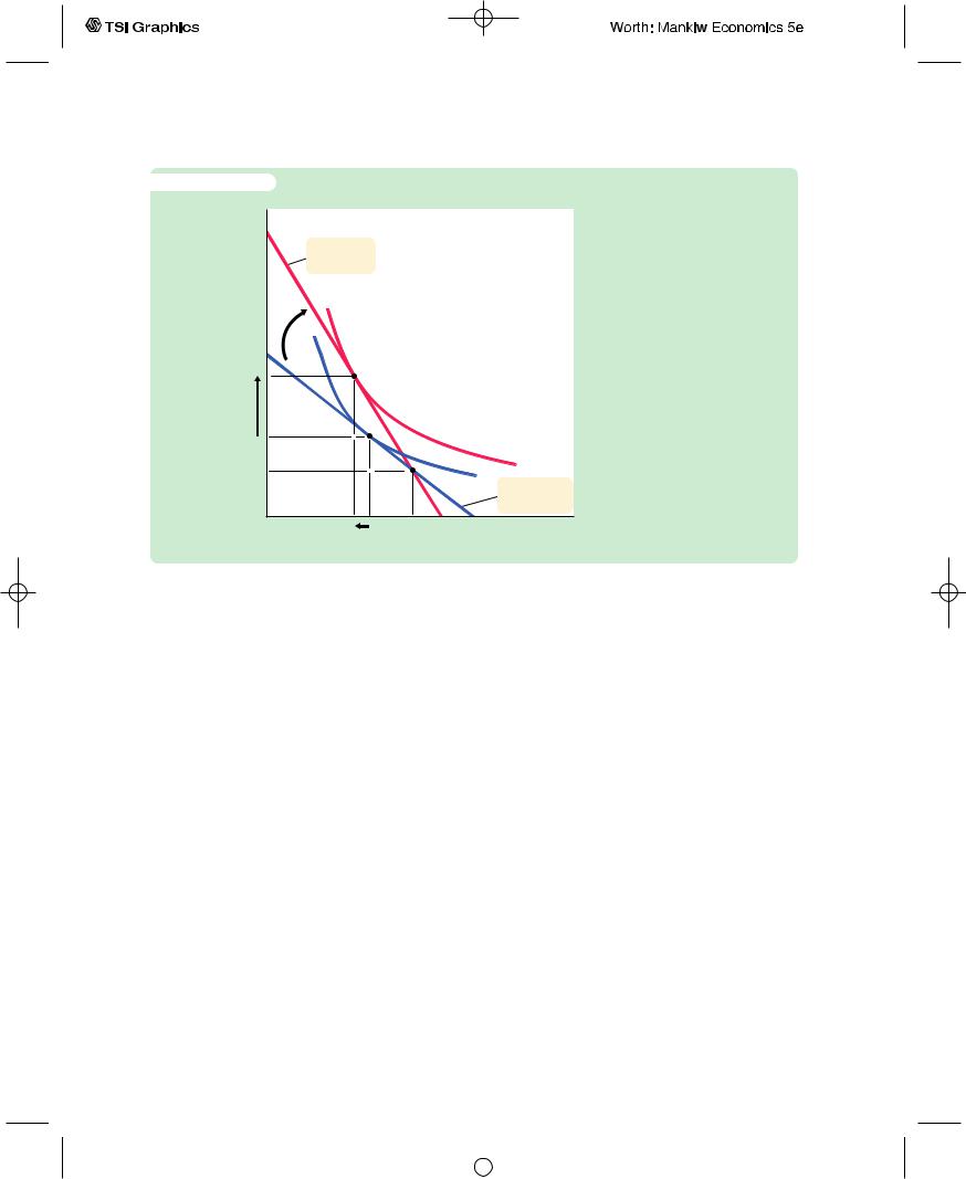
Figure 16-7 shows that an increase in the real interest rate rotates the consumer’s budget line around the point (Y1, Y2) and, thereby, alters the amount of consumption he chooses in both periods. Here, the consumer moves from point A to point B.You can see that for the indifference curves drawn in this figure first-period consumption falls and second-period consumption rises.

Economists decompose the impact of an increase in the real interest rate on consumption into two effects: an income effect and a substitution effect.Textbooks in microeconomics discuss these effects in detail.We summarize them briefly here.

The income effect is the change in consumption that results from the movement to a higher indifference curve. Because the consumer is a saver rather than a borrower (as indicated by the fact that first-period consumption is less than firstperiod income), the increase in the interest rate makes him better off (as reflected by the movement to a higher indifference curve). If consumption in period one and consumption in period two are both normal goods, the consumer will want to spread this improvement in his welfare over both periods. This income effect tends to make the consumer want more consumption in both periods.

The substitution effect is the change in consumption that results from the change in the relative price of consumption in the two periods. In particular, consumption in period two becomes less expensive relative to consumption in period one when the interest rate rises. That is, because the real interest rate earned on saving is higher, the consumer must now give up less first-period consumption to obtain an extra unit of second-period consumption. This substitution effect tends to make the consumer choose more consumption in period two and less consumption in period one.

The consumer’s choice depends on both the income effect and the substitution effect. Both effects act to increase the amount of second-period consumption;

hence, we can confidently conclude that an increase in the real interest rate raises second-period consumption. But the two effects have opposite impacts on firstperiod consumption, so the increase in the interest rate could either raise or lower it. Hence, depending on the relative size of the income and substitution effects, an increase in the interest rate could either stimulate or depress saving.

Constraints on Borrowing

Fisher’s model assumes that the consumer can borrow as well as save.The ability to borrow allows current consumption to exceed current income. In essence, when the consumer borrows, he consumes some of his future income today.Yet for many people such borrowing is impossible. For example, a student wishing to enjoy spring break in Florida would probably be unable to finance this vacation with a bank loan. Let’s examine how Fisher’s analysis changes if the consumer cannot borrow.

The inability to borrow prevents current consumption from exceeding current income.A constraint on borrowing can therefore be expressed as

C1 ≤ Y1.

This inequality states that consumption in period one must be less than or equal to income in period one. This additional constraint on the consumer is called a borrowing constraint or, sometimes, a liquidity constraint.

C H A P T E R 1 6 Consumption | 445

f i g u r e 1 6 - 8

446 | P A R T V I More on the Microeconomics Behind Macroeconomics

The Consumer’s Optimum With a Borrowing Constraint When the consumer faces a borrowing constraint, there are two possible situations. In panel (a), the consumer chooses first-period consumption to be less than first-period income, so the borrowing constraint is not binding and does not affect consumption in either period. In panel (b), the borrowing constraint is binding. The consumer would like to borrow and choose point D. But because borrowing is not allowed, the best available choice is point E. When the borrowing constraint is binding, first-period consumption equals first-period income.

C A S E S T U D Y

The High Japanese Saving Rate

Japan has one of the world’s highest saving rates, and this fact is important for understanding both the long-run and short-run performance of its economy. On the one hand, many economists believe that the high Japanese saving rate is a key to the rapid growth Japan experienced in the decades after World War II. Indeed, the Solow growth model developed in Chapters 7 and 8 shows that the saving rate is a primary determinant of a country’s steadystate level of income. On other other hand, some economists have argued that the high Japanese saving rate contributed to Japan’s slump during the 1990s. High saving means low consumer spending, which according to the IS–LM model of Chapters 10 and 11 translates into low aggregate demand and reduced income.

Why do the Japanese consume a much smaller fraction of their income than Americans? One reason is that it is harder for households to borrow in

C H A P T E R 1 6 Consumption | 447

Japan. As Fisher’s model shows, a household facing a binding borrowing constraint consumes less than it would without the borrowing constraint. Hence, societies in which borrowing constraints are common will tend to have higher rates of saving.

One reason that households often wish to borrow is to buy a home. In the United States, a person can usually buy a home with a down payment of 10 percent. A homebuyer in Japan cannot borrow nearly this much: down payments of 40 percent are common. Moreover, housing prices are very high in Japan, primarily because land prices are high. A Japanese family must save a great deal if it is ever to afford its own home.

Although constraints on borrowing are part of the explanation of high Japanese saving, there are many other differences between Japan and the United States that contribute to the difference in the saving rates.The Japanese tax system encourages saving by taxing capital income very lightly. In addition, cultural differences may lead to differences in consumer preferences regarding present and future consumption. One prominent Japanese economist writes, “The Japanese are simply different.They are more risk averse and more patient. If this is true, the long-run implication is that Japan will absorb all the wealth in the world. I refuse to comment on this explanation.’’1

16-3 Franco Modigliani and the

Life-Cycle Hypothesis

In a series of papers written in the 1950s, Franco Modigliani and his collaborators Albert Ando and Richard Brumberg used Fisher’s model of consumer behavior to study the consumption function. One of their goals was to solve the consumption puzzle—that is, to explain the apparently conflicting pieces of evidence that came to light when Keynes’s consumption function was brought to the data. According to Fisher’s model, consumption depends on a person’s lifetime income. Modigliani emphasized that income varies systematically over people’s lives and that saving allows consumers to move income from those times in life when income is high to those times when it is low. This interpretation of consumer behavior formed the basis for his life-cycle hypothesis.2

1Fumio Hayashi,“Why Is Japan’s Saving Rate So Apparently High?’’ NBER Macroeconomics Annual (1986): 147–210.

2For references to the large body of work on the life-cycle hypothesis, a good place to start is the lecture Modigliani gave when he won the Nobel Prize. Franco Modigliani,“Life Cycle, Individual Thrift, and the Wealth of Nations,’’ American Economic Review 76 ( June 1986): 297–313.

448 | P A R T V I More on the Microeconomics Behind Macroeconomics

The Hypothesis

One important reason that income varies over a person’s life is retirement. Most people plan to stop working at about age 65, and they expect their incomes to fall when they retire.Yet they do not want a large drop in their standard of living, as measured by their consumption. To maintain consumption after retirement, people must save during their working years. Let’s see what this motive for saving implies for the consumption function.

Consider a consumer who expects to live another T years, has wealth of W, and expects to earn income Y until she retires R years from now.What level of consumption will the consumer choose if she wishes to maintain a smooth level of consumption over her life?

The consumer’s lifetime resources are composed of initial wealth W and lifetime earnings of R × Y. (For simplicity, we are assuming an interest rate of zero; if the interest rate were greater than zero, we would need to take account of interest earned on savings as well.) The consumer can divide up her lifetime resources among her T remaining years of life. We assume that she wishes to achieve the smoothest possible path of consumption over her lifetime.Therefore, she divides this total of W + RY equally among the T years and each year consumes

C = (W + RY )/T.

We can write this person’s consumption function as

C = (1/T )W + (R/T )Y.

For example, if the consumer expects to live for 50 more years and work for 30 of them, then T = 50 and R = 30, so her consumption function is

C = 0.02W + 0.6Y.

This equation says that consumption depends on both income and wealth. An extra $1 of income per year raises consumption by $0.60 per year, and an extra $1 of wealth raises consumption by $0.02 per year.

If every individual in the economy plans consumption like this, then the aggregate consumption function is much the same as the individual one. In particular, aggregate consumption depends on both wealth and income. That is, the economy’s consumption function is

C = aW + bY,

where the parameter a is the marginal propensity to consume out of wealth, and the parameter b is the marginal propensity to consume out of income.

Implications

Figure 16-10 graphs the relationship between consumption and income predicted by the life-cycle model. For any given level of wealth W, the model yields a conventional consumption function similar to the one shown in Figure 16-1.