Mankiw Macroeconomics (5th ed)

C H A P T E R 1 4 Stabilization Policy | 399

ployment, the average growth of real GDP, or the volatility of real GDP. Central-bank independence appears to offer countries a free lunch: it has the benefit of lower inflation without any apparent cost.This finding has led some countries, such as New Zealand, to rewrite their laws to give their central banks greater independence.8

14-3 Conclusion: Making Policy in an

Uncertain World

In this chapter we have examined whether policy should take an active or passive role in responding to economic fluctuations and whether policy should be conducted by rule or by discretion.There are many arguments on both sides of these questions. Perhaps the only clear conclusion is that there is no simple and compelling case for any particular view of macroeconomic policy. In the end, you must weigh the various arguments, both economic and political, and decide for yourself what kind of role the government should play in trying to stabilize the economy.

For better or worse, economists play a key role in the formulation of economic policy. Because the economy is complex, this role is often difficult.Yet it is also inevitable. Economists cannot sit back and wait until our knowledge of the economy has been perfected before giving advice. In the meantime, someone must advise economic policymakers.That job, difficult as it sometimes is, falls to economists.

The role of economists in the policymaking process goes beyond giving advice to policymakers. Even economists cloistered in academia influence policy indirectly through their research and writing. In the conclusion of The General Theory, John Maynard Keynes wrote that

the ideas of economists and political philosophers, both when they are right and when they are wrong, are more powerful than is commonly understood. Indeed, the world is ruled by little else. Practical men, who believe themselves to be quite exempt from intellectual influences, are usually the slaves of some defunct economist. Madmen in authority, who hear voices in the air, are distilling their frenzy from some academic scribbler of a few years back.

This is as true today as it was when Keynes wrote it in 1936—except now that academic scribbler is often Keynes himself.

8 For a more complete presentation of these findings and references to the large literature on central-bank independence, see Alberto Alesina and Lawrence H. Summers, “Central Bank Independence and Macroeconomic Performance: Some Comparative Evidence,” Journal of Money, Credit, and Banking 25 (May 1993): 151–162. For a study that questions the link between inflation and central-bank independence, see Marta Campillo and Jeffrey A. Miron, “Why Does Inflation Differ Across Countries?” in Christina D. Romer and David H. Romer, eds., Reducing Inflation: Motivation and Strategy (Chicago: University of Chicago Press, 1997), 335–362.

400 | P A R T V Macroeconomic Policy Debates

Summary

1.Advocates of active policy view the economy as subject to frequent shocks that will lead to unnecessary fluctuations in output and employment unless monetary or fiscal policy responds. Many believe that economic policy has been successful in stabilizing the economy.

2.Advocates of passive policy argue that because monetary and fiscal policies work with long and variable lags, attempts to stabilize the economy are likely to end up being destabilizing. In addition, they believe that our present understanding of the economy is too limited to be useful in formulating successful stabilization policy and that inept policy is a frequent source of economic fluctuations.

3.Advocates of discretionary policy argue that discretion gives more flexibility to policymakers in responding to various unforeseen situations.

4.Advocates of policy rules argue that the political process cannot be trusted. They believe that politicians make frequent mistakes in conducting economic policy and sometimes use economic policy for their own political ends. In addition, advocates of policy rules argue that a commitment to a fixed policy rule is necessary to solve the problem of time inconsistency.

K E Y C O N C E P T S

Q U E S T I O N S F O R R E V I E W

C H A P T E R 1 4 Stabilization Policy | 401

P R O B L E M S A N D A P P L I C A T I O N S

402 | P A R T V Macroeconomic Policy Debates

A P P E N D I X

Time Inconsistency and the Tradeoff Between

Inflation and Unemployment

In this appendix, we examine more analytically the time-inconsistency argument for rules rather than discretion.This material is relegated to an appendix because we will need to use some calculus.9

Suppose that the Phillips curve describes the relationship between inflation and unemployment. Letting u denote the unemployment rate, un the natural rate of unemployment, p the rate of inflation, and pe the expected rate of inflation, unemployment is determined by

u = un − a(p − pe).

Unemployment is low when inflation exceeds expected inflation and high when inflation falls below expected inflation.The parameter a determines how much unemployment responds to surprise inflation.

For simplicity, suppose also that the Fed chooses the rate of inflation. Of course, more realistically, the Fed controls inflation only imperfectly through its control of the money supply. But for purposes of illustration, it is useful to assume that the Fed can control inflation perfectly.

The Fed likes low unemployment and low inflation. Suppose that the cost of unemployment and inflation, as perceived by the Fed, can be represented as

L(u, p) = u + gp2,

where the parameter g represents how much the Fed dislikes inflation relative to unemployment. L(u, p) is called the loss function. The Fed’s objective is to make the loss as small as possible.

Having specified how the economy works and the Fed’s objective, let’s compare monetary policy made under a fixed rule and under discretion.

First, consider policy under a fixed rule.A rule commits the Fed to a particular level of inflation. As long as private agents understand that the Fed is committed to this rule, the expected level of inflation will be the level the Fed is committed to produce. Because expected inflation equals actual inflation (pe = p), unemployment will be at its natural rate (u = un).

What is the optimal rule? Because unemployment is at its natural rate regardless of the level of inflation legislated by the rule, there is no benefit to having any inflation at all. Therefore, the optimal fixed rule requires that the Fed produce zero inflation.

9 The material in this appendix is derived from Finn E. Kydland and Edward C. Prescott, “Rules Rather Than Discretion:The Inconsistency of Optimal Plans,’’ Journal of Political Economy 85 ( June 1977): 473–492; and Robert J. Barro and David Gordon,“A Positive Theory of Monetary Policy in a Natural Rate Model,’’ Journal of Political Economy 91 (August 1983): 589–610.

C H A P T E R 1 4 Stabilization Policy | 403

Second, consider discretionary monetary policy. Under discretion, the economy works as follows:

1.Private agents form their expectations of inflation pe.

2.The Fed chooses the actual level of inflation p.

3.Based on expected and actual inflation, unemployment is determined.

Under this arrangement, the Fed minimizes its loss L(u, p) subject to the constraint that the Phillips curve imposes.When making its decision about the rate of inflation, the Fed takes expected inflation as already determined.

To find what outcome we would obtain under discretionary policy, we must examine what level of inflation the Fed would choose. By substituting the Phillips curve into the Fed’s loss function, we obtain

L(u, p) = un − a(p − pe) + gp2.

Notice that the Fed’s loss is negatively related to unexpected inflation (the second term in the equation) and positively related to actual inflation (the third term).To find the level of inflation that minimizes this loss, differentiate with respect to p to obtain

dL/dp = −a + 2gp.

The loss is minimized when this derivative equals zero. Solving for p, we get p = a/(2g).

Whatever level of inflation private agents expected, this is the “optimal’’ level of inflation for the Fed to choose. Of course, rational private agents understand the objective of the Fed and the constraint that the Phillips curve imposes. They therefore expect that the Fed will choose this level of inflation. Expected inflation equals actual inflation [pe = p = a/(2g)], and unemployment equals its natural rate (u = un).

Now compare the outcome under optimal discretion to the outcome under the optimal rule. In both cases, unemployment is at its natural rate.Yet discretionary policy produces more inflation than does policy under the rule. Thus, optimal discretion is worse than the optimal rule.This is true even though the Fed under discretion was attempting to minimize its loss, L(u, p).

At first it may seem strange that the Fed can achieve a better outcome by being committed to a fixed rule. Why can’t the Fed with discretion mimic the Fed committed to a zero-inflation rule? The answer is that the Fed is playing a game against private decisionmakers who have rational expectations. Unless it is committed to a fixed rule of zero inflation, the Fed cannot get private agents to expect zero inflation.

Suppose, for example, that the Fed simply announces that it will follow a zeroinflation policy. Such an announcement by itself cannot be credible.After private agents have formed their expectations of inflation, the Fed has the incentive to renege on its announcement in order to decrease unemployment. (As we have

404 | P A R T V Macroeconomic Policy Debates

just seen, once expectations are given, the Fed’s optimal policy is to set inflation at p = a/(2g), regardless of pe.) Private agents understand the incentive to renege and therefore do not believe the announcement in the first place.

This theory of monetary policy has an important corollary. Under one circumstance, the Fed with discretion achieves the same outcome as the Fed committed to a fixed rule of zero inflation. If the Fed dislikes inflation much more than it dislikes unemployment (so that g is very large), inflation under discretion is near zero, because the Fed has little incentive to inflate. This finding provides some guidance to those who have the job of appointing central bankers. An alternative to imposing a fixed rule is to appoint an individual with a fervent distaste for inflation. Perhaps this is why even liberal politicians ( Jimmy Carter, Bill Clinton) who are more concerned about unemployment than inflation sometimes appoint conservative central bankers (Paul Volcker, Alan Greenspan) who are more concerned about inflation.

M O R E P R O B L E M S A N D A P P L I C A T I O N S

C H A P T1E R 5 F I F T E E N

Government Debt

Blessed are the young, for they shall inherit the national debt.

— Herbert Hoover

When a government spends more than it collects in taxes, it borrows from the private sector to finance the budget deficit.The accumulation of past borrowing is the government debt. Debate about the appropriate amount of government debt in the United States is as old as the country itself. Alexander Hamilton believed that “a national debt, if it is not excessive, will be to us a national blessing,” whereas James Madison argued that “a public debt is a public curse.” Indeed, the location of the nation’s capital was chosen as part of a deal in which the federal government assumed the Revolutionary War debts of the states: because the Northern states had larger outstanding debts, the capital was located in the South.

Although attention to the government debt has waxed and waned over the years, it was especially intense during the last two decades of the twentieth century. Beginning in the early 1980s, the U.S. federal government began running large budget deficits—in part because of increased spending and in part because of reduced taxes. As a result, the government debt expressed as a percentage of GDP roughly doubled from 26 percent in 1980 to 50 percent in 1995. By the late 1990s, the budget deficit had come under control and had even turned into a budget surplus. Policymakers then turned to the question of how rapidly the debt should be paid off.

The large increase in government debt from 1980 to 1995 is without precedent in U.S. history. Government debt most often rises in periods of war or depression, but the United States experienced neither during this time. Not surprisingly, the episode sparked a renewed interest among economists and policymakers in the economic effects of government debt. Some view the large budget deficits of the 1980s and 1990s as the worst mistake of economic policy since the Great Depression, whereas others think that the deficits matter very little. This chapter considers various facets of this debate.

We begin by looking at the numbers. Section 15-1 examines the size of the U.S. government debt, comparing it to the debt of other countries and to the debt that the United States has had during its own past. It also takes a brief look at what the future may hold. Section 15-2 discusses why measuring changes in

| 405

406 | P A R T V Microeconomic Policy Debates

government indebtedness is not as straightforward as it might seem. Indeed, some economists argue that traditional measures are so misleading that they should be completely ignored.

We then look at how government debt affects the economy. Section 15-3 describes the traditional view of government debt, according to which government borrowing reduces national saving and crowds out capital accumulation. This view is held by most economists and has been implicit in the discussion of fiscal policy throughout this book. Section 15-4 discusses an alternative view, called Ricardian equivalence, which is held by a small but influential minority of economists. According to the Ricardian view, government debt does not influence national saving and capital accumulation. As we will see, the debate between the traditional and Ricardian views of government debt arises from disagreements over how consumers respond to the government’s debt policy.

Section 15-5 then looks at other facets of the debate over government debt. It begins by discussing whether the government should try to always balance its budget and, if not, when a budget deficit or surplus is desirable. It also examines the effects of government debt on monetary policy, the political process, and the role of a country in the world economy.

15-1 The Size of the Government Debt

Let’s begin by putting the government debt in perspective. In 2001, the debt of the U.S. federal government was $3.2 trillion. If we divide this number by 276 million, the number of people in the United States, we find that each person’s share of the government debt was about $11,600. Obviously, this is not a trivial number—few people sneeze at $11,600.Yet if we compare this debt to

t a b l e 1 5 - 1

How Indebted Are the World’s Governments?

Source: OECD Economic Outlook. Figures are based on estimates of gross government debt and GDP for 2001.

C H A P T E R 1 5 Government Debt | 407

the roughly $1 million a typical person will earn over his or her working life, the government debt does not look like the catastrophe it is sometimes made out to be.

One way to judge the size of a government’s debt is to compare it to the amount of debt other countries have accumulated.Table 15-1 shows the amount of government debt for 19 major countries expressed as a percentage of each country’s GDP. On the top of the list are the heavily indebted countries of Japan and Italy, which have accumulated a debt that exceeds annual GDP. At the bottom are Norway and Australia, which have accumulated relatively small debts. The United States is in the middle of the pack. By international standards, the U.S. government is neither especially profligate nor especially frugal.

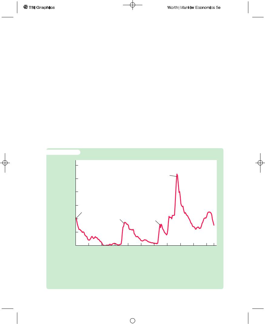
Over the course of U.S. history, the indebtedness of the federal government has varied substantially. Figure 15-1 shows the ratio of the federal debt to GDP since 1791.The government debt, relative to the size of the economy, varies from close to zero in the 1830s to a maximum of 107 percent of GDP in 1945.

Historically, the primary cause of increases in the government debt is war. The debt–GDP ratio rises sharply during major wars and falls slowly during peacetime. Many economists think that this historical pattern is the appropriate

The Ratio of Government Debt to GDP Since 1790 The U.S. federal government debt held by the public, relative to the size of the U.S. economy, rises sharply during wars and declines slowly during peacetime. The exception is the period since 1980, when the debt–GDP ratio rose without the occurrence of a major military conflict.

Source: U.S. Department of Treasury, U.S. Department of Commerce, and T.S. Berry, “Production and Population Since 1789,” Bostwick Paper No. 6, Richmond, 1988.

408 | P A R T V Microeconomic Policy Debates

way to run fiscal policy. As we discuss more fully later in this chapter, deficit financing of wars appears optimal for reasons of both tax smoothing and generational equity. One instance of a large increase in government debt in peacetime occurred during the 1980s and early 1990s, when the federal government ran substantial budget deficits. Many economists have criticized this increase in government debt as imposing a burden on future generations without justification.

During the middle of the 1990s, the U.S. federal government started to get its budget deficit under control. A combination of tax hikes, spending cuts, and rapid economic growth caused the ratio of debt to GDP to stabilize and then decline. Recent experience has tempted some observers to think that exploding government debt is a thing of the past. But as the next case study suggests, the worst may be yet to come.

C A S E S T U D Y

The Fiscal Future: Good News and Bad News

What does the future hold for fiscal policymakers? Economic forecasting is far from precise, and it is easy to be cynical about economic predictions. But good policy cannot be made if policymakers only look backwards. As a result, economists in the Congressional Budget Office (CBO) and other government agencies are always trying to look ahead to see what problems and opportunities are likely to develop.

When George W. Bush moved into the White House in 2001, the fiscal picture facing the U.S. government was mixed. In particular, it depended on how far one looked ahead.

Over a tenor twenty-year horizon, the picture looked good.The U.S. federal government was running a large budget surplus. As a percentage of GDP, the projected surplus for 2001 was the largest since 1948. Moreover, the surplus was expected to grow even larger over time. The surplus was large enough so that, without any policy changes, the government debt would be paid off by 2008.

These surpluses arose from various sources.The elder George Bush had signed a tax increase in 1990, and Bill Clinton had signed another in 1993. Because of these tax hikes, federal tax revenue as a percentage of GDP reached its highest level since World War II. Then, in the late 1990s, productivity accelerated, most likely because of advances in information technology. The high growth in incomes led to rising tax revenue, which pushed the federal government’s budget from deficit to surplus.

A debate arose over how to respond to the budget surplus. The government could use the large projected surpluses to repay debt, increase spending, cut taxes, or some combination of these. The new Republican president George W. Bush advocated a tax cut of $1.6 trillion over 10 years, which was about one-fourth of the projected surpluses. Democrats in Congress argued for a smaller tax cut and greater government spending.The end result was a compromise bill that cut taxes by a bit less than Bush had advocated.