Mankiw Macroeconomics (5th ed)

C H A P T E R 1 3 Aggregate Supply | 359

the previous year’s price level, means higher inflation.Thus, when policymakers move the economy up along the short-run aggregate supply curve, they reduce the unemployment rate and raise the inflation rate. Conversely, when they contract aggregate demand and move the economy down the short-run aggregate supply curve, unemployment rises and inflation falls.

This tradeoff between inflation and unemployment, called the Phillips curve, is our topic in this section. As we have just seen (and will derive more formally in a moment), the Phillips curve is a reflection of the short-run aggregate supply curve: as policymakers move the economy along the short-run aggregate supply curve, unemployment and inflation move in opposite directions. The Phillips curve is a useful way to express aggregate supply because inflation and unemployment are such important measures of economic performance.

Deriving the Phillips Curve From the Aggregate

Supply Curve

The Phillips curve in its modern form states that the inflation rate depends on three forces:

Expected inflation;

The deviation of unemployment from the natural rate, called cyclical unemployment;

Supply shocks.

These three forces are expressed in the following equation:

where b is a parameter measuring the response of inflation to cyclical unemployment. Notice that there is a minus sign before the cyclical unemployment term: high unemployment tends to reduce inflation.This equation summarizes the relationship between inflation and unemployment.

From where does this equation for the Phillips curve come? Although it may not seem familiar, we can derive it from our equation for aggregate supply.To see how, write the aggregate supply equation as

With one addition, one subtraction, and one substitution, we can manipulate this equation to yield a relationship between inflation and unemployment.

Here are the three steps. First, add to the right-hand side of the equation a supply shock u to represent exogenous events (such as a change in world oil prices) that alter the price level and shift the short-run aggregate supply curve:

360 | P A R T I V Business Cycle Theory: The Economy in the Short Run

Next, to go from the price level to inflation rates, subtract last year’s price level P−1 from both sides of the equation to obtain

The term on the left-hand side, P − P−1, is the difference between the current price level and last year’s price level, which is inflation p.8 The term on the right-hand side, Pe − P−1, is the difference between the expected price level and last year’s price level, which is expected inflation pe.Therefore, we can replace P − P−1 with p and Pe − P−1 with pe:

Third, to go from output to unemployment, recall from Chapter 2 that Okun’s law gives a relationship between these two variables. One version of Okun’s law states that the deviation of output from its natural rate is inversely related to the deviation of unemployment from its natural rate; that is, when output is higher than the natural rate of output, unemployment is lower than the natural rate of unemployment.We can write this as

p = pe − b(u − un) + u.

Thus, we can derive the Phillips curve equation from the aggregate supply equation.

All this algebra is meant to show one thing: the Phillips curve equation and the short-run aggregate supply equation represent essentially the same macroeconomic ideas. In particular, both equations show a link between real and nominal variables that causes the classical dichotomy (the theoretical separation of real and nominal variables) to break down in the short run. According to the short-run aggregate supply equation, output is related to unexpected movements in the price level. According to the Phillips curve equation, unemployment is related to unexpected movements in the inflation rate.The aggregate supply curve is more convenient when we are studying output and the price level, whereas the Phillips curve is more convenient when we are studying unemployment and inflation. But we should not lose sight of the fact that the Phillips curve and the aggregate supply curve are two sides of the same coin.

8 Mathematical note: This statement is not precise, because inflation is really the percentage change in the price level.To make the statement more precise, interpret P as the logarithm of the price level. By the properties of logarithms, the change in P is roughly the inflation rate. The reason is that dP = d(log price level) = d(price level)/price level.

C H A P T E R 1 3 Aggregate Supply | 361

FYIThe History of the Modern Phillips Curve

Adaptive Expectations and Inflation Inertia

To make the Phillips curve useful for analyzing the choices facing policymakers, we need to say what determines expected inflation. A simple and often plausible assumption is that people form their expectations of inflation based on recently observed inflation.This assumption is called adaptive expectations. For example, suppose that people expect prices to rise this year at the same rate as they did last year.Then expected inflation pe equals last year’s inflation p−1:

pe = p−1.

In this case, we can write the Phillips curve as

p = p−1 − b(u − un) + u,

which states that inflation depends on past inflation, cyclical unemployment, and a supply shock.When the Phillips curve is written in this form, the natural rate of unemployment is sometimes called the Non-Accelerating Inflation Rate of Unemployment, or NAIRU.

The first term in this form of the Phillips curve, p−1, implies that inflation has inertia.That is, like an object moving through space, inflation keeps going unless something acts to stop it. In particular, if unemployment is at the NAIRU and if there are no supply shocks, the continued rise in price level neither speeds up nor slows down.This inertia arises because past inflation influences expectations of future inflation and because these expectations influence the wages and prices

9 A. W. Phillips, “The Relationship Between Unemployment and the Rate of Change of Money Wages in the United Kingdom, 1861–1957,’’ Economica 25 (November 1958): 283–299.

362 | P A R T I V Business Cycle Theory: The Economy in the Short Run

that people set. Robert Solow captured the concept of inflation inertia well when, during the high inflation of the 1970s, he wrote,“Why is our money ever less valuable? Perhaps it is simply that we have inflation because we expect inflation, and we expect inflation because we’ve had it.’’

In the model of aggregate supply and aggregate demand, inflation inertia is interpreted as persistent upward shifts in both the aggregate supply curve and the aggregate demand curve. Consider first aggregate supply. If prices have been rising quickly, people will expect them to continue to rise quickly. Because the position of the short-run aggregate supply curve depends on the expected price level, the short-run aggregate supply curve will shift upward over time. It will continue to shift upward until some event, such as a recession or a supply shock, changes inflation and thereby changes expectations of inflation.

The aggregate demand curve must also shift upward to confirm the expectations of inflation. Most often, the continued rise in aggregate demand is caused by persistent growth in the money supply. If the Fed suddenly halted money growth, aggregate demand would stabilize, and the upward shift in aggregate supply would cause a recession.The high unemployment in the recession would reduce inflation and expected inflation, causing inflation inertia to subside.

Two Causes of Rising and Falling Inflation

The second and third terms in the Phillips curve equation show the two forces that can change the rate of inflation.

The second term, b(u − un), shows that cyclical unemployment—the deviation of unemployment from its natural rate—exerts upward or downward pressure on inflation. Low unemployment pulls the inflation rate up. This is called demand-pull inflation because high aggregate demand is responsible for this type of inflation. High unemployment pulls the inflation rate down.The parameter b measures how responsive inflation is to cyclical unemployment.

The third term, u, shows that inflation also rises and falls because of supply shocks. An adverse supply shock, such as the rise in world oil prices in the 1970s, implies a positive value of u and causes inflation to rise. This is called cost-push inflation because adverse supply shocks are typically events that push up the costs of production. A beneficial supply shock, such as the oil glut that led to a fall in oil prices in the 1980s, makes u negative and causes inflation to fall.

C A S E S T U D Y

Inflation and Unemployment in the United States

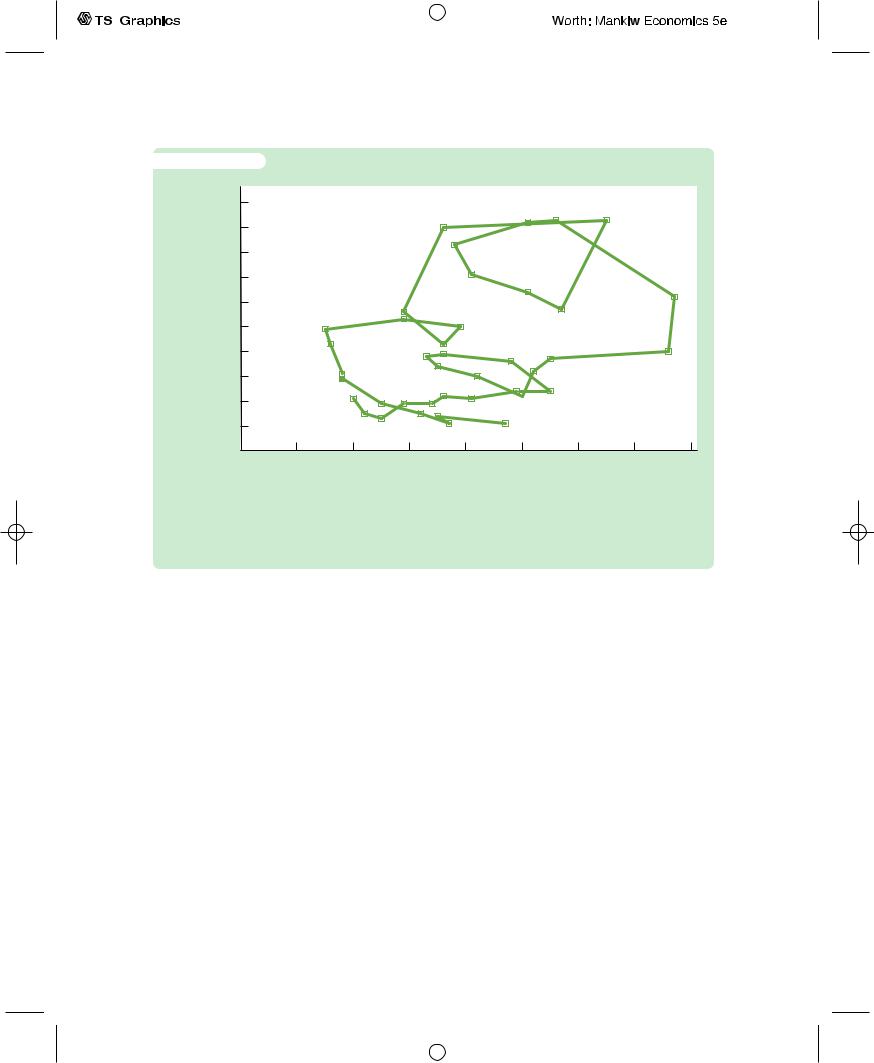
Because inflation and unemployment are such important measures of economic performance, macroeconomic developments are often viewed through the lens of the Phillips curve. Figure 13-5 displays the history of inflation and unemployment in the United States since 1961.These four decades of data illustrate some of the causes of rising or falling inflation.

Unemployment (percent)

Inflation and Unemployment in the United States Since 1961 This figure uses annual data on the unemployment rate and the inflation rate (percentage change in the GDP deflator) to illustrate macroeconomic developments over the past four decades.

Source: U.S. Department of Commerce and U.S. Department of Labor.

The 1960s showed how policymakers can, in the short run, lower unemployment at the cost of higher inflation.The tax cut of 1964, together with expansionary monetary policy, expanded aggregate demand and pushed the unemployment rate below 5 percent.This expansion of aggregate demand continued in the late 1960s largely as a by-product of government spending for the Vietnam War. Unemployment fell lower and inflation rose higher than policymakers intended.

The 1970s were a period of economic turmoil.The decade began with policymakers trying to lower the inflation inherited from the 1960s. President Nixon imposed temporary controls on wages and prices, and the Federal Reserve engineered a recession through contractionary monetary policy, but the inflation rate fell only slightly.The effects of wage and price controls ended when the controls were lifted, and the recession was too small to counteract the inflationary impact of the boom that had preceded it. By 1972 the unemployment rate was the same as a decade earlier, whereas inflation was 3 percentage points higher.

Beginning in 1973 policymakers had to cope with the large supply shocks caused by the Organization of Petroleum Exporting Countries (OPEC). OPEC first raised oil prices in the mid-1970s, pushing the inflation rate up to about 10 percent.This adverse supply shock, together with temporarily tight monetary policy, led to a recession in 1975. High unemployment during the recession reduced inflation somewhat, but further OPEC price hikes pushed inflation up again in the late 1970s.

364 | P A R T I V Business Cycle Theory: The Economy in the Short Run

The 1980s began with high inflation and high expectations of inflation. Under the leadership of Chairman Paul Volcker, the Federal Reserve doggedly pursued monetary policies aimed at reducing inflation. In 1982 and 1983 the unemployment rate reached its highest level in 40 years. High unemployment, aided by a fall in oil prices in 1986, pulled the inflation rate down from about 10 percent to about 3 percent. By 1987 the unemployment rate of about 6 percent was close to most estimates of the natural rate. Unemployment continued to fall through the 1980s, however, reaching a low of 5.2 percent in 1989 and beginning a new round of demand-pull inflation.

Compared to the previous 30 years, the 1990s were relatively quiet. The decade began with a recession caused by several contractionary shocks to aggregate demand: tight monetary policy, the savings-and-loan crisis, and a fall in consumer confidence coinciding with the Gulf War.The unemployment rate rose to 7.3 percent in 1992. Inflation fell, but only slightly. Unlike in the 1982 recession, unemployment in the 1990 recession was never far above the natural rate, so the effect on inflation was small.

By the late 1990s, inflation and unemployment both reached their lowest levels in many years. Some economists explain this fortunate development by claiming that the economy’s natural rate of unemployment fell (for reasons discussed in Chapter 6). Others argue that various temporary factors (such as a strong U.S. dollar attributable to a financial crisis in Asia) yielded favorable supply shocks. Most likely, a combination of events helped keep inflation in check, despite low unemployment. In 2000, however, inflation did begin to creep up.

Thus, U.S. macroeconomic history exhibits the many causes of inflation.The 1960s and the 1980s show the two sides of demand-pull inflation: in the 1960s low unemployment pulled inflation up, and in the 1980s high unemployment pulled inflation down. The 1970s with their oil-price hikes show the effects of cost-push inflation.

The Short-Run Tradeoff Between

Inflation and Unemployment

Consider the options the Phillips curve gives to a policymaker who can influence aggregate demand with monetary or fiscal policy.At any moment, expected inflation and supply shocks are beyond the policymaker’s immediate control.Yet, by changing aggregate demand, the policymaker can alter output, unemployment, and inflation.The policymaker can expand aggregate demand to lower unemployment and raise inflation. Or the policymaker can depress aggregate demand to raise unemployment and lower inflation.

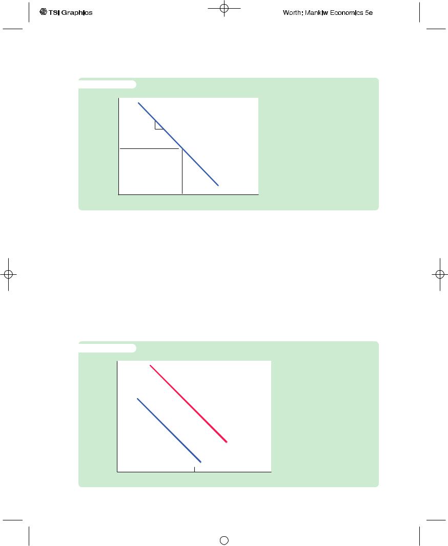
Figure 13-6 plots the Phillips curve equation and shows the short-run tradeoff between inflation and unemployment. When unemployment is at its natural rate (u = un), inflation depends on expected inflation and the supply shock (p = pe + u). The parameter b determines the slope of the tradeoff between inflation and unemployment. In the short run, for a given level of expected inflation, policymakers can manipulate aggregate demand to choose a

combination of inflation and unemployment on this curve, called the short-run Phillips curve.

Notice that the position of the short-run Phillips curve depends on the expected rate of inflation. If expected inflation rises, the curve shifts upward, and the policymaker’s tradeoff becomes less favorable: inflation is higher for any level of unemployment. Figure 13-7 shows how the tradeoff depends on expected inflation.

Because people adjust their expectations of inflation over time, the tradeoff between inflation and unemployment holds only in the short run.The policymaker cannot keep inflation above expected inflation (and thus unemployment below its natural rate) forever. Eventually, expectations adapt to whatever inflation rate the

High expected inflation

Low expected inflation

366 | P A R T I V Business Cycle Theory: The Economy in the Short Run

FYIHow Precise Are Estimates of the Natural Rate

of Unemployment?

policymaker has chosen. In the long run, the classical dichotomy holds, unemployment returns to its natural rate, and there is no tradeoff between inflation and unemployment.

Disinflation and the Sacrifice Ratio

Imagine an economy in which unemployment is at its natural rate and inflation is running at 6 percent.What would happen to unemployment and output if the central bank pursued a policy to reduce inflation from 6 to 2 percent?

The Phillips curve shows that in the absence of a beneficial supply shock, lowering inflation requires a period of high unemployment and reduced output. But by how much and for how long would unemployment need to rise above the natural rate? Before deciding whether to reduce inflation, policymakers must know how much output would be lost during the transition to lower inflation. This cost can then be compared with the benefits of lower inflation.

10 Douglas Staiger, James H. Stock, and Mark W.Watson,“How Precise Are Estimates of the Natural Rate of Unemployment?” in Christina D. Romer and David H. Romer, eds., Reducing Inflation: Motivation and Strategy (Chicago: University of Chicago Press, 1997).

C H A P T E R 1 3 Aggregate Supply | 367

Much research has used the available data to examine the Phillips curve quantitatively.The results of these studies are often summarized in a number called the sacrifice ratio, the percentage of a year’s real GDP that must be forgone to reduce inflation by 1 percentage point. Although estimates of the sacrifice ratio vary substantially, a typical estimate is about 5: for every percentage point that inflation is to fall, 5 percent of one year’s GDP must be sacrificed.11

We can also express the sacrifice ratio in terms of unemployment. Okun’s law says that a change of 1 percentage point in the unemployment rate translates into a change of 2 percentage points in GDP. Therefore, reducing inflation by 1 percentage point requires about 2.5 percentage points of cyclical unemployment.

We can use the sacrifice ratio to estimate by how much and for how long unemployment must rise to reduce inflation. If reducing inflation by 1 percentage point requires a sacrifice of 5 percent of a year’s GDP, reducing inflation by 4 percentage points requires a sacrifice of 20 percent of a year’s GDP. Equivalently, this reduction in inflation requires a sacrifice of 10 percentage points of cyclical unemployment.

This disinflation could take various forms, each totaling the same sacrifice of 20 percent of a year’s GDP. For example, a rapid disinflation would lower output by 10 percent for 2 years: this is sometimes called the cold-turkey solution to inflation. A moderate disinflation would lower output by 5 percent for 4 years. An even more gradual disinflation would depress output by 2 percent for a decade.

Rational Expectations and the Possibility

of Painless Disinflation

Because the expectation of inflation influences the short-run tradeoff between inflation and unemployment, it is crucial to understand how people form expectations. So far, we have been assuming that expected inflation depends on recently observed inflation. Although this assumption of adaptive expectations is plausible, it is probably too simple to apply in all circumstances.

An alternative approach is to assume that people have rational expectations. That is, we might assume that people optimally use all the available information, including information about current government policies, to forecast the future. Because monetary and fiscal policies influence inflation, expected inflation should also depend on the monetary and fiscal policies in effect. According to the theory of rational expectations, a change in monetary or fiscal policy will change expectations, and an evaluation of any policy change must incorporate this effect on expectations. If people do form their expectations rationally, then inflation may have less inertia than it first appears.

11 Arthur M. Okun, “Efficient Disinflationary Policies,’’ American Economic Review 68 (May 1978): 348–352; and Robert J. Gordon and Stephen R. King,“The Output Cost of Disinflation in Traditional andVector Autoregressive Models,’’ Brookings Papers on Economic Activity (1982:1): 205–245.

368 | P A R T I V Business Cycle Theory: The Economy in the Short Run

Here is how Thomas Sargent, a prominent advocate of rational expectations, describes its implications for the Phillips curve:

An alternative “rational expectations’’ view denies that there is any inherent momentum to the present process of inflation.This view maintains that firms and workers have now come to expect high rates of inflation in the future and that they strike inflationary bargains in light of these expectations. However, it is held that people expect high rates of inflation in the future precisely because the government’s current and prospective monetary and fiscal policies warrant those expectations. . . .Thus inflation only seems to have a momentum of its own; it is actually the long-term government policy of persistently running large deficits and creating money at high rates which imparts the momentum to the inflation rate.An implication of this view is that inflation can be stopped much more quickly than advocates of the “momentum’’ view have indicated and that their estimates of the length of time and the costs of stopping inflation in terms of foregone output are erroneous. . . . [Stopping inflation] would require a change in the policy regime: there must be an abrupt change in the continuing government policy, or strategy, for setting deficits now and in the future that is sufficiently binding as to be widely believed. . . . How costly such a move would be in terms of foregone output and how long it would be in taking effect would depend partly on how resolute and evident the government’s commitment was.12

Thus, advocates of rational expectations argue that the short-run Phillips curve does not accurately represent the options that policymakers have available. They believe that if policymakers are credibly committed to reducing inflation, rational people will understand the commitment and will quickly lower their expectations of inflation. Inflation can then come down without a rise in unemployment and fall in output. According to the theory of rational expectations, traditional estimates of the sacrifice ratio are not useful for evaluating the impact of alternative policies. Under a credible policy, the costs of reducing inflation may be much lower than estimates of the sacrifice ratio suggest.

In the most extreme case, one can imagine reducing the rate of inflation without causing any recession at all.A painless disinflation has two requirements. First, the plan to reduce inflation must be announced before the workers and firms who set wages and prices have formed their expectations. Second, the workers and firms must believe the announcement; otherwise, they will not reduce their expectations of inflation. If both requirements are met, the announcement will immediately shift the short-run tradeoff between inflation and unemployment downward, permitting a lower rate of inflation without higher unemployment.

Although the rational-expectations approach remains controversial, almost all economists agree that expectations of inflation influence the short-run tradeoff between inflation and unemployment.The credibility of a policy to reduce inflation is therefore one determinant of how costly the policy will be. Unfortunately, it is often difficult to predict whether the public will view the announcement of a new policy as credible.The central role of expectations makes forecasting the results of alternative policies far more difficult.

12 Thomas J. Sargent,“The Ends of Four Big Inflations,’’ in Robert E. Hall, ed., Inflation: Causes and Effects (Chicago: University of Chicago Press, 1982).