Mankiw Macroeconomics (5th ed)

C H A P T E R 1 3 Aggregate Supply | 349

The Sticky-Wage Model

To explain why the short-run aggregate supply curve is upward sloping, many economists stress the sluggish adjustment of nominal wages. In many industries, nominal wages are set by long-term contracts, so wages cannot adjust quickly when economic conditions change. Even in industries not covered by formal contracts, implicit agreements between workers and firms may limit wage changes. Wages may also depend on social norms and notions of fairness that evolve slowly. For these reasons, many economists believe that nominal wages are sticky in the short run.

The sticky-wage model shows what a sticky nominal wage implies for aggregate supply. To preview the model, consider what happens to the amount of output produced when the price level rises:

1.When the nominal wage is stuck, a rise in the price level lowers the real wage, making labor cheaper.

2.The lower real wage induces firms to hire more labor.

3.The additional labor hired produces more output.

This positive relationship between the price level and the amount of output means that the aggregate supply curve slopes upward during the time when the nominal wage cannot adjust.

To develop this story of aggregate supply more formally, assume that workers and firms bargain over and agree on the nominal wage before they know what the price level will be when their agreement takes effect. The bargaining par- ties—the workers and the firms—have in mind a target real wage.The target may be the real wage that equilibrates labor supply and demand. More likely, the target real wage is higher than the equilibrium real wage: as discussed in Chapter 6, union power and efficiency-wage considerations tend to keep real wages above the level that brings supply and demand into balance.

The workers and firms set the nominal wage W based on the target real wage q and on their expectation of the price level P e.The nominal wage they set is

W = q × P e

Nominal Wage = Target Real Wage × Expected Price Level.

After the nominal wage has been set and before labor has been hired, firms learn the actual price level P.The real wage turns out to be

W/P = q × (P e/P)

Expected Price Level

Real Wage = Target Real Wage × .

Actual Price Level

This equation shows that the real wage deviates from its target if the actual price level differs from the expected price level.When the actual price level is greater than expected, the real wage is less than its target; when the actual price level is less than expected, the real wage is greater than its target.

350 | P A R T I V Business Cycle Theory: The Economy in the Short Run

The final assumption of the sticky-wage model is that employment is determined by the quantity of labor that firms demand. In other words, the bargain between the workers and the firms does not determine the level of employment in advance; instead, the workers agree to provide as much labor as the firms wish to buy at the predetermined wage.We describe the firms’ hiring decisions by the labor demand function

L = Ld(W/P ),

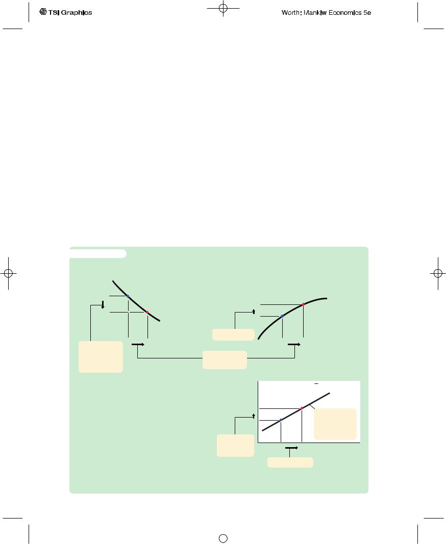
which states that the lower the real wage, the more labor firms hire. The labor demand curve is shown in panel (a) of Figure 13-1. Output is determined by the production function

Y = F(L),

which states that the more labor is hired, the more output is produced. This is shown in panel (b) of Figure 13-1.

Panel (c) of Figure 13-1 shows the resulting aggregate supply curve. Because the nominal wage is sticky, an unexpected change in the price level

C H A P T E R 1 3 Aggregate Supply | 351

moves the real wage away from the target real wage, and this change in the real wage influences the amounts of labor hired and output produced. The aggregate supply curve can be written as

Output deviates from its natural level when the price level deviates from the expected price level.1

C A S E S T U D Y

The Cyclical Behavior of the Real Wage

In any model with an unchanging labor demand curve, such as the model we just discussed, employment rises when the real wage falls. In the sticky-wage model, an unexpected rise in the price level lowers the real wage and thereby raises the quantity of labor hired and the amount of output produced.Thus, the real wage should be countercyclical: it should fluctuate in the opposite direction from employment and output. Keynes himself wrote in The General Theory that “an increase in employment can only occur to the accompaniment of a decline in the rate of real wages.’’

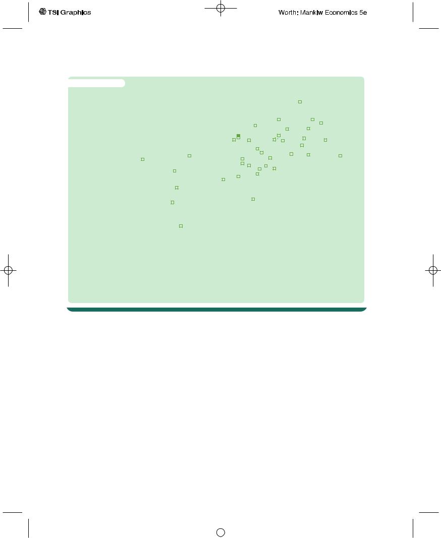
The earliest attacks on The General Theory came from economists challenging Keynes’s prediction. Figure 13-2 is a scatterplot of the percentage change in real compensation per hour and the percentage change in real GDP using annual data for the U.S. economy from 1960 to 2000. If Keynes’s prediction were correct, the dots in this figure would show a downward-sloping pattern, indicating a negative relationship.Yet the figure shows only a weak correlation between the real wage and output, and it is the opposite of what Keynes predicted.That is, if the real wage is cyclical at all, it is slightly procyclical: the real wage tends to rise when output rises. Abnormally high labor costs cannot explain the low employment and output observed in recessions.

How should we interpret this evidence? Most economists conclude that the sticky-wage model cannot fully explain aggregate supply.They advocate models in which the labor demand curve shifts over the business cycle.These shifts may arise because firms have sticky prices and cannot sell all they want at those prices; we discuss this possibility later. Alternatively, the labor demand curve may shift because of shocks to technology, which alter labor productivity.The theory we discuss in Chapter 19, called the theory of real business cycles, gives a prominent role to technology shocks as a source of economic fluctuations.2

1For more on the sticky-wage model, see Jo Anna Gray,“Wage Indexation:A Macroeconomic Approach,’’ Journal of Monetary Economics 2 (April 1976): 221–235; and Stanley Fischer, “Long-Term Contracts, Rational Expectations, and the Optimal Money Supply Rule,’’ Journal of Political Economy 85 (February 1977): 191–205.

2For some of the recent work on the cyclical behavior of the real wage, see Scott Sumner and

Stephen Silver, “Real Wages, Employment, and the Phillips Curve,’’ Journal of Political Economy 97 ( June 1989): 706–720; and Gary Solon, Robert Barsky, and Jonathan A. Parker, “Measuring the Cyclicality of Real Wages: How Important Is Composition Bias?’’ Quarterly Journal of Economics 109 (February 1994): 1–25.

352 | P A R T I V Business Cycle Theory: The Economy in the Short Run

f i g u r e 1 3 - 2

Percentage change in real GDP

The Cyclical Behavior of the Real Wage This scatterplot shows the percentage change in real GDP and the percentage change in the real wage (measured here as real private hourly earnings). As output fluctuates, the real wage typically moves in the same direction. That is, the real wage is somewhat procyclical. This observation is inconsistent with the sticky-wage model.

Source: U.S. Department of Commerce and U.S. Department of Labor.

The Imperfect-Information Model

The second explanation for the upward slope of the short-run aggregate supply curve is called the imperfect-information model. Unlike the sticky-wage model, this model assumes that markets clear—that is, all wages and prices are free to adjust to balance supply and demand. In this model, the short-run and long-run aggregate supply curves differ because of temporary misperceptions about prices.

The imperfect-information model assumes that each supplier in the economy produces a single good and consumes many goods. Because the number of goods is so large, suppliers cannot observe all prices at all times. They monitor closely the prices of what they produce but less closely the prices of all the goods they consume. Because of imperfect information, they sometimes confuse changes in the overall level of prices with changes in relative prices. This confusion influences decisions about how much to supply, and it leads to a positive relationship between the price level and output in the short run.

Consider the decision facing a single supplier—a wheat farmer, for instance. Because the farmer earns income from selling wheat and uses this income to buy goods and services, the amount of wheat she chooses to produce depends on the

C H A P T E R 1 3 Aggregate Supply | 353

price of wheat relative to the prices of other goods and services in the economy. If the relative price of wheat is high, the farmer is motivated to work hard and produce more wheat, because the reward is great. If the relative price of wheat is low, she prefers to enjoy more leisure and produce less wheat.

Unfortunately, when the farmer makes her production decision, she does not know the relative price of wheat. As a wheat producer, she monitors the wheat market closely and always knows the nominal price of wheat. But she does not know the prices of all the other goods in the economy. She must, therefore, estimate the relative price of wheat using the nominal price of wheat and her expectation of the overall price level.

Consider how the farmer responds if all prices in the economy, including the price of wheat, increase. One possibility is that she expected this change in prices. When she observes an increase in the price of wheat, her estimate of its relative price is unchanged. She does not work any harder.

The other possibility is that the farmer did not expect the price level to increase (or to increase by this much).When she observes the increase in the price of wheat, she is not sure whether other prices have risen (in which case wheat’s relative price is unchanged) or whether only the price of wheat has risen (in which case its relative price is higher).The rational inference is that some of each has happened. In other words, the farmer infers from the increase in the nominal price of wheat that its relative price has risen somewhat. She works harder and produces more.

Our wheat farmer is not unique.When the price level rises unexpectedly, all suppliers in the economy observe increases in the prices of the goods they produce.They all infer, rationally but mistakenly, that the relative prices of the goods they produce have risen.They work harder and produce more.

To sum up, the imperfect-information model says that when actual prices exceed expected prices, suppliers raise their output. The model implies an aggre-

Output deviates from the natural rate when the price level deviates from the expected price level.3

The Sticky-Price Model

Our third explanation for the upward-sloping short-run aggregate supply curve is called the sticky-price model.This model emphasizes that firms do not instantly adjust the prices they charge in response to changes in demand. Sometimes prices are set by long-term contracts between firms and customers. Even

3 Two economists who have emphasized the role of imperfect information for understanding the short-run effects of monetary policy are the Nobel Prize winners Milton Friedman and Robert Lucas. See Milton Friedman,“The Role of Monetary Policy,’’ American Economic Review 58 (March 1968): 1–17; and Robert E. Lucas, Jr.,“Understanding Business Cycles,’’ Stabilization of the Domestic and International Economy, vol. 5 of Carnegie-Rochester Conference on Public Policy (Amsterdam: North-Holland, 1977).

354 | P A R T I V Business Cycle Theory: The Economy in the Short Run

without formal agreements, firms may hold prices steady in order not to annoy their regular customers with frequent price changes. Some prices are sticky because of the way markets are structured: once a firm has printed and distributed its catalog or price list, it is costly to alter prices.

To see how sticky prices can help explain an upward-sloping aggregate supply curve, we first consider the pricing decisions of individual firms and then add together the decisions of many firms to explain the behavior of the economy as a whole. Notice that this model encourages us to depart from the assumption of perfect competition, which we have used since Chapter 3. Perfectly competitive firms are price takers rather than price setters. If we want to consider how firms set prices, it is natural to assume that these firms have at least some monopoly control over the prices they charge.

Consider the pricing decision facing a typical firm.The firm’s desired price p depends on two macroeconomic variables:

The overall level of prices P. A higher price level implies that the firm’s costs are higher. Hence, the higher the overall price level, the more the firm would like to charge for its product.

The level of aggregate income Y. A higher level of income raises the demand for the firm’s product. Because marginal cost increases at higher levels of production, the greater the demand, the higher the firm’s desired price.

We write the firm’s desired price as

= + − − p P a(Y Y ).

This equation says that the desired price p depends on the overall level of prices

− −

P and on the level of aggregate output relative to the natural rate Y Y .The parameter a (which is greater than zero) measures how much the firm’s desired price responds to the level of aggregate output.4

Now assume that there are two types of firms. Some have flexible prices: they always set their prices according to this equation. Others have sticky prices: they announce their prices in advance based on what they expect economic conditions to be. Firms with sticky prices set prices according to

where, as before, a superscript “e’’ represents the expected value of a variable. For

p = P e.

That is, firms with sticky prices set their prices based on what they expect other firms to charge.

4 Mathematical note: The firm cares most about its relative price, which is the ratio of its nominal price to the overall price level. If we interpret p and P as the logarithms of the firm’s price and the price level, then this equation states that the desired relative price depends on the deviation of output from the natural rate.

C H A P T E R 1 3 Aggregate Supply | 355

We can use the pricing rules of the two groups of firms to derive the aggregate supply equation.To do this, we find the overall price level in the economy, which is the weighted average of the prices set by the two groups. If s is the fraction of firms with sticky prices and 1 − s the fraction with flexible prices, then the overall price level is

The first term is the price of the sticky-price firms weighted by their fraction in the economy, and the second term is the price of the flexible-price firms weighted by their fraction. Now subtract (1 − s)P from both sides of this equation to obtain

Divide both sides by s to solve for the overall price level:

The two terms in this equation are explained as follows:

When firms expect a high price level, they expect high costs.Those firms that fix prices in advance set their prices high.These high prices cause the other firms to set high prices also. Hence, a high expected price level P e leads to a high actual price level P.

When output is high, the demand for goods is high.Those firms with flexible prices set their prices high, which leads to a high price level.The effect of output on the price level depends on the proportion of firms with flexible prices.

Hence, the overall price level depends on the expected price level and on the level of output.

Algebraic rearrangement puts this aggregate pricing equation into a more familiar form:

where a = s/[(1 − s)a]. Like the other models, the sticky-price model says that the deviation of output from the natural rate is positively associated with the deviation of the price level from the expected price level.

Although the sticky-price model emphasizes the goods market, consider briefly what is happening in the labor market. If a firm’s price is stuck in the short run, then a reduction in aggregate demand reduces the amount that the firm is able to sell.The firm responds to the drop in sales by reducing its production and its demand for labor. Note the contrast to the sticky-wage model: the firm here does not move along a fixed labor demand curve. Instead, fluctuations in output are associated with shifts in the labor demand curve. Because of these shifts in labor demand, employment, production, and the real wage can all move in the same direction.Thus, the real wage can be procyclical.5

5 For a more advanced development of the sticky-price model, see Julio Rotemberg,“Monopolistic Price Adjustment and Aggregate Output,’’ Review of Economic Studies 49 (1982): 517–531.

356 | P A R T I V Business Cycle Theory: The Economy in the Short Run

C A S E S T U D Y

International Differences in the Aggregate Supply Curve

Although all countries experience economic fluctuations, these fluctuations are not exactly the same everywhere. International differences are intriguing puzzles in themselves, and they often provide a way to test alternative economic theories. Examining international differences has been especially fruitful in research on aggregate supply.

When economist Robert Lucas proposed the imperfect-information model, he derived a surprising interaction between aggregate demand and aggregate supply: according to his model, the slope of the aggregate supply curve should depend on the volatility of aggregate demand. In countries where aggregate demand fluctuates widely, the aggregate price level fluctuates widely as well. Because most movements in prices in these countries do not represent movements in relative prices, suppliers should have learned not to respond much to unexpected changes in the price level. Therefore, the aggregate supply curve should be relatively steep (that is, a will be small). Conversely, in countries where aggregate demand is relatively stable, suppliers should have learned that most price changes are relative price changes.Accordingly, in these countries, suppliers should be more responsive to unexpected price changes, making the aggregate supply curve relatively flat (that is, a will be large).

Lucas tested this prediction by examining international data on output and prices. He found that changes in aggregate demand have the biggest effect on output in those countries where aggregate demand and prices are most stable. Lucas concluded that the evidence supports the imperfect-information model.6 The sticky-price model also makes predictions about the slope of the shortrun aggregate supply curve. In particular, it predicts that the average rate of inflation should influence the slope of the short-run aggregate supply curve. When the average rate of inflation is high, it is very costly for firms to keep prices fixed for long intervals.Thus, firms adjust prices more frequently. More frequent price adjustment in turn allows the overall price level to respond more quickly to shocks to aggregate demand. Hence, a high rate of inflation should make the

short-run aggregate supply curve steeper.

International data support this prediction of the sticky-price model. In countries with low average inflation, the short-run aggregate supply curve is relatively flat: fluctuations in aggregate demand have large effects on output and are slowly reflected in prices. High-inflation countries have steep short-run aggregate supply curves. In other words, high inflation appears to erode the frictions that cause prices to be sticky.7

Note that the sticky-price model can also explain Lucas’s finding that countries with variable aggregate demand have steep aggregate supply curves. If the price level is highly variable, few firms will commit to prices in advance (s will be small). Hence, the aggregate supply curve will be steep (a will be small).

6Robert E. Lucas, Jr.,“Some International Evidence on Output-Inflation Tradeoffs,’’ American Economic Review 63 ( June 1973): 326–334.

7Laurence Ball, N. Gregory Mankiw, and David Romer,“The New Keynesian Economics and the Output-Inflation Tradeoff,’’ Brookings Papers on Economic Activity (1988:1): 1–65.

C H A P T E R 1 3 Aggregate Supply | 357

Summary and Implications

We have seen three models of aggregate supply and the market imperfection that each uses to explain why the short-run aggregate supply curve is upward sloping. One model assumes nominal wages are sticky; the second assumes information about prices is imperfect; the third assumes prices are sticky. Keep in mind that these models are not incompatible with one another. We need not accept one model and reject the others.The world may contain all three of these market imperfections, and all may contribute to the behavior of short-run aggregate supply.

Although the three models of aggregate supply differ in their assumptions and emphases, their implications for aggregate output are similar. All can be summarized by the equation

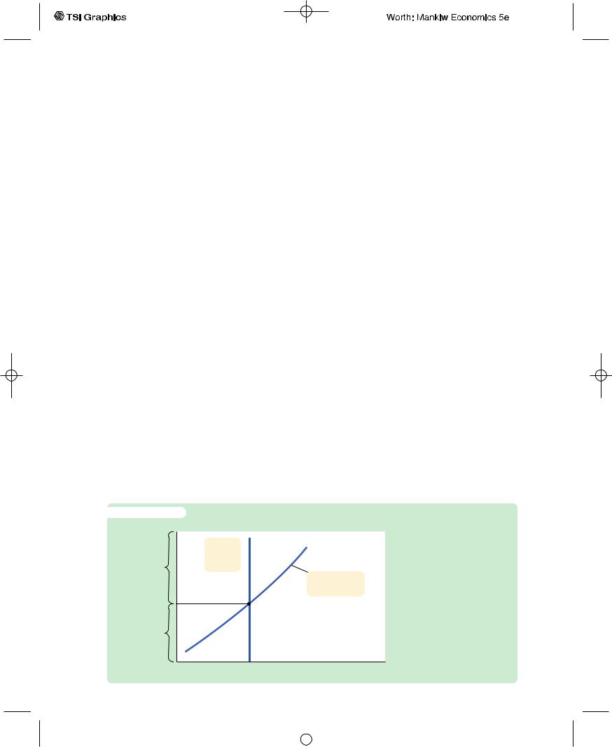
This equation states that deviations of output from the natural rate are related to deviations of the price level from the expected price level. If the price level is higher than the expected price level, output exceeds its natural rate. If the price level is lower than the expected price level, output falls short of its natural rate. Figure 13-3 graphs this equation. Notice that the short-run aggregate supply curve is drawn for a given expectation P e and that a change in P e would shift the curve.

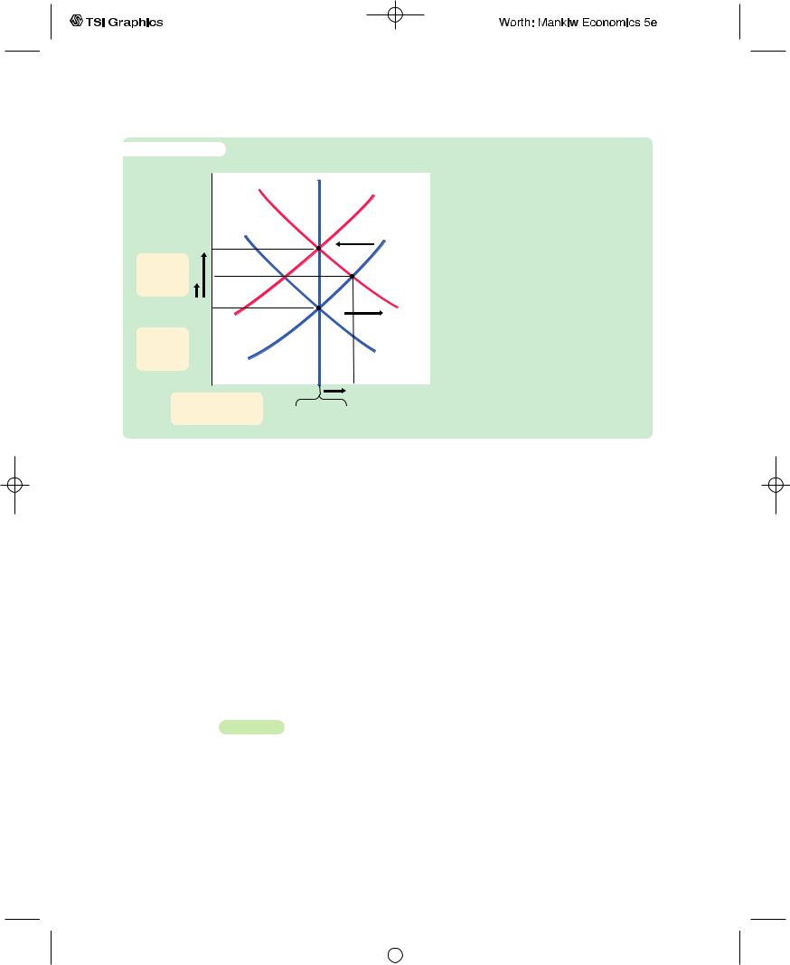
Now that we have a better understanding of aggregate supply, let’s put aggregate supply and aggregate demand back together. Figure 13-4 uses our aggregate supply equation to show how the economy responds to an unexpected increase in aggregate demand attributable, say, to an unexpected monetary expansion. In the short run, the equilibrium moves from point A to point B. The increase in aggregate demand raises the actual price level from P1 to P2. Because people did not expect this increase in the price level, the expected price level

remains at Pe, and output rises from Y to Y , which is above the natural rate

− 2 1 2

Y . Thus, the unexpected expansion in aggregate demand causes the economy to boom.

P < Pe

358 | P A R T I V Business Cycle Theory: The Economy in the Short Run

Yet the boom does not last forever. In the long run, the expected price level rises to catch up with reality, causing the short-run aggregate supply curve to shift upward. As the expected price level rises from P2e to P3e, the equilibrium of the economy moves from point B to point C.The actual price level rises from P2 to P3, and output falls from Y2 to Y3. In other words, the economy returns to the natural level of output in the long run, but at a much higher price level.

This analysis shows an important principle, which holds for each of the three models of aggregate supply: long-run monetary neutrality and short-run monetary nonneutrality are perfectly compatible. Short-run nonneutrality is represented here by the movement from point A to point B, and long-run monetary neutrality is represented by the movement from point A to point C.We reconcile the short-run and long-run effects of money by emphasizing the adjustment of expectations about the price level.

13-2 Inflation, Unemployment, and the

Phillips Curve

Two goals of economic policymakers are low inflation and low unemployment, but often these goals conflict. Suppose, for instance, that policymakers were to use monetary or fiscal policy to expand aggregate demand. This policy would move the economy along the short-run aggregate supply curve to a point of higher output and a higher price level. (Figure 13-4 shows this as the change from point A to point B.) Higher output means lower unemployment, because firms need more workers when they produce more. A higher price level, given