Mankiw Macroeconomics (5th ed)

C H A P T E R 1 2 Aggregate Demand in the Open Economy | 339

currency to appreciate, reducing net exports and offsetting the usual expansionary impact on aggregate income. Fiscal policy does influence aggregate income under fixed exchange rates.

3.The Mundell–Fleming model shows that monetary policy does not influence aggregate income under fixed exchange rates. Any attempt to expand the money supply is futile, because the money supply must adjust to ensure that the exchange rate stays at its announced level. Monetary policy does influence aggregate income under floating exchange rates.

4.If investors are wary of holding assets in a country, the interest rate in that country may exceed the world interest rate by some risk premium.According to the Mundell–Fleming model, an increase in the risk premium causes the interest rate to rise and the currency of that country to depreciate.

5.There are advantages to both floating and fixed exchange rates. Floating exchange rates leave monetary policymakers free to pursue objectives other than exchange-rate stability. Fixed exchange rates reduce some of the uncertainty in international business transactions.

K E Y C O N C E P T S

Q U E S T I O N S F O R R E V I E W

P R O B L E M S A N D A P P L I C A T I O N S

340 | P A R T I V Business Cycle Theory: The Economy in the Short Run

C H A P T E R 1 2 Aggregate Demand in the Open Economy | 341

A P P E N D I X

A Short-Run Model of the Large Open Economy

When analyzing policies in an economy such as the United States, we need to combine the closed-economy logic of the IS–LM model and the small-open- economy logic of the Mundell–Fleming model.This appendix presents a model for the intermediate case of a large open economy.

As we discussed in the appendix to Chapter 5, a large open economy differs from a small open economy because its interest rate is not fixed by world financial markets. In a large open economy, we must consider the relationship between the interest rate and the flow of capital abroad. The net capital outflow is the amount that domestic investors lend abroad minus the amount that foreign investors lend here. As the domestic interest rate falls, domestic investors find foreign lending more attractive, and foreign investors find lending here less attractive.Thus, the net capital outflow is negatively related to the interest rate. Here we add this relationship to our short-run model of national income.

The three equations of the model are

Y = C(Y − T ) + I(r) + G + NX(e),

M/P = L(r, Y ),

NX(e) = CF(r).

The first two equations are the same as those used in the Mundell–Fleming model of this chapter.The third equation, taken from the appendix to Chapter 5, states that the trade balance NX equals the net capital outflow CF, which in turn depends on the domestic interest rate.

To see what this model implies, substitute the third equation into the first, so the model becomes

These two equations are much like the two equations of the closed-economy IS–LM model.The only difference is that expenditure now depends on the interest rate for two reasons. As before, a higher interest rate reduces investment. But now, a higher interest rate also reduces the net capital outflow and thus lowers net exports.

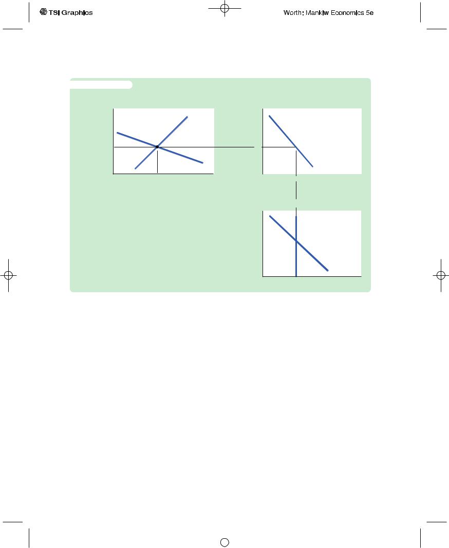
To analyze this model, we can use the three graphs in Figure 12-14 on page 342. Panel (a) shows the IS–LM diagram. As in the closed-economy model in Chapters 10 and 11, the interest rate r is on the vertical axis, and income Y is on the horizontal axis. The IS and LM curves together determine the equilibrium level of income and the equilibrium interest rate.

342 | P A R T I V Business Cycle Theory: The Economy in the Short Run

The new net-capital-outflow term in the IS equation, CF(r), makes this IS curve flatter than it would be in a closed economy.The more responsive international capital flows are to the interest rate, the flatter the IS curve is.You might recall from the Chapter 5 appendix that the small open economy represents the extreme case in which the net capital outflow is infinitely elastic at the world interest rate. In this extreme case, the IS curve is completely flat. Hence, a small open economy would be depicted in this figure with a horizontal IS curve.

Panels (b) and (c) show how the equilibrium from the IS–LM model determines the net capital outflow, the trade balance, and the exchange rate. In panel

(b) we see that the interest rate determines the net capital outflow. This curve slopes downward because a higher interest rate discourages domestic investors from lending abroad and encourages foreign investors to lend here. In panel (c) we see that the exchange rate adjusts to ensure that net exports of goods and services equal the net capital outflow.

Now let’s use this model to examine the impact of various policies.We assume that the economy has a floating exchange rate, because this assumption is correct for most large open economies such as the United States.

C H A P T E R 1 2 Aggregate Demand in the Open Economy | 343

Fiscal Policy

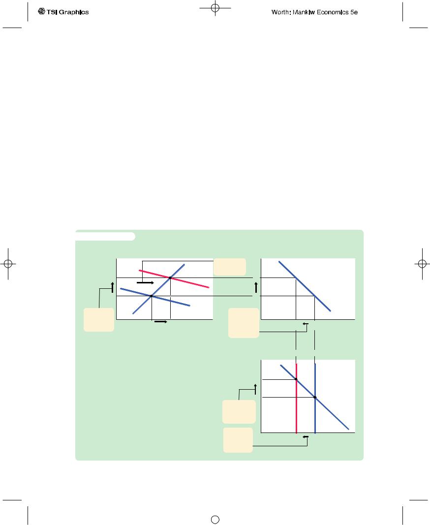
Figure 12-15 examines the impact of a fiscal expansion. An increase in government purchases or a cut in taxes shifts the IS curve to the right. As panel (a) illustrates, this shift in the IS curve leads to an increase in the level of income and an increase in the interest rate. These two effects are similar to those in a closed economy.

Yet, in the large open economy, the higher interest rate reduces the net capital outflow, as in panel (b).The fall in the net capital outflow reduces the supply of dollars in the market for foreign exchange. The exchange rate appreciates, as in panel (c). Because domestic goods become more expensive relative to foreign goods, net exports fall.

Figure 12-15 shows that a fiscal expansion does raise income in the large open economy, unlike in a small open economy under a floating exchange rate. The impact on income, however, is smaller than in a closed economy. In a closed economy, the expansionary impact of fiscal policy is partially offset by the

f i g u r e 1 2 - 1 5

(c) The Market for Foreign Exchange

344 | P A R T I V Business Cycle Theory: The Economy in the Short Run

crowding out of investment: as the interest rate rises, investment falls, reducing the fiscal-policy multipliers. In a large open economy, there is yet another offsetting factor: as the interest rate rises, the net capital outflow falls, the exchange rate appreciates, and net exports fall. Together these effects are not large enough to make fiscal policy powerless, as it is in a small open economy, but they do reduce fiscal policy’s impact.

Monetary Policy

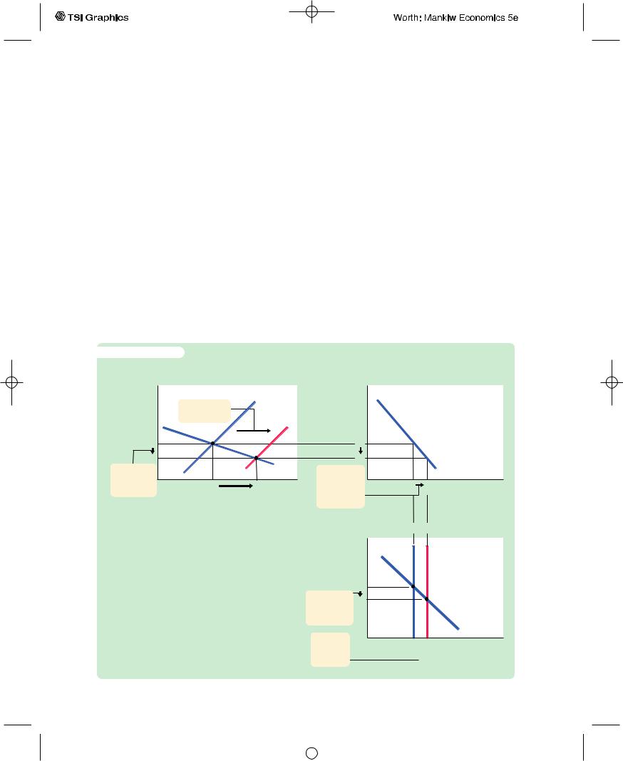
Figure 12-16 examines the effect of a monetary expansion. An increase in the money supply shifts the LM curve to the right, as in panel (a). The level of income rises, and the interest rate falls. Once again, these effects are similar to those in a closed economy.

Yet, as panel (b) shows, the lower interest rate leads to a higher net capital outflow.The increase in CF raises the supply of dollars in the market for foreign exchange.The exchange rate depreciates, as in panel (c).As domestic goods become cheaper relative to foreign goods, net exports rise.

f i g u r e 1 2 - 1 6

C H A P T E R 1 2 Aggregate Demand in the Open Economy | 345

We can now see that the monetary transmission mechanism has two parts in a large open economy. As in a closed economy, a monetary expansion lowers the interest rate. As in a small open economy, a monetary expansion causes the currency to depreciate in the market for foreign exchange. The lower interest rate stimulates investment, and the lower exchange rate stimulates net exports.

A Rule of Thumb

This model of the large open economy describes well the U.S. economy today. Yet it is somewhat more complicated and cumbersome than the model of the closed economy we studied in Chapters 10 and 11 and the model of the small open economy we developed in this chapter. Fortunately, there is a useful rule of thumb to help you determine how policies influence a large open economy without remembering all the details of the model: The large open economy is an average of the closed economy and the small open economy.To find how any policy will affect any variable, find the answer in the two extreme cases and take an average.

For example, how does a monetary contraction affect the interest rate and investment in the short run? In a closed economy, the interest rate rises, and investment falls. In a small open economy, neither the interest rate nor investment changes.The effect in the large open economy is an average of these two cases: a monetary contraction raises the interest rate and reduces investment, but only somewhat.The fall in the net capital outflow mitigates the rise in the interest rate and the fall in investment that would occur in a closed economy. But unlike in a small open economy, the international flow of capital is not so strong as to negate fully these effects.

This rule of thumb makes the simple models all the more valuable. Although they do not describe perfectly the world in which we live, they do provide a useful guide to the effects of economic policy.

M O R E P R O B L E M S A N D A P P L I C A T I O N S

346 | P A R T I V Business Cycle Theory: The Economy in the Short Run

C H A P T1E R 3 T H I R T E E N

Aggregate Supply

There is always a temporary tradeoff between inflation and unemploy-

ment; there is no permanent tradeoff. The temporary tradeoff comes not

from inflation per se, but from unanticipated inflation, which generally

means, from a rising rate of inflation.

— Milton Friedman

Most economists analyze short-run fluctuations in aggregate income and the price level using the model of aggregate demand and aggregate supply. In the previous three chapters, we examined aggregate demand in some detail. The IS–LM model—together with its open-economy cousin the Mundell–Fleming model—shows how changes in monetary and fiscal policy and shocks to the money and goods markets shift the aggregate demand curve. In this chapter, we turn our attention to aggregate supply and develop theories that explain the position and slope of the aggregate supply curve.

When we introduced the aggregate supply curve in Chapter 9, we established that aggregate supply behaves differently in the short run than in the long run. In the long run, prices are flexible, and the aggregate supply curve is vertical.When the aggregate supply curve is vertical, shifts in the aggregate demand curve affect the price level, but the output of the economy remains at its natural rate. By contrast, in the short run, prices are sticky, and the aggregate supply curve is not vertical. In this case, shifts in aggregate demand do cause fluctuations in output. In Chapter 9 we took a simplified view of price stickiness by drawing the short-run aggregate supply curve as a horizontal line, representing the extreme situation in which all prices are fixed. Our task now is to refine this understanding of shortrun aggregate supply.

Unfortunately, one fact makes this task more difficult: economists disagree about how best to explain aggregate supply. As a result, this chapter begins by presenting three prominent models of the short-run aggregate supply curve. Among economists, each of these models has some prominent adherents (as well as some prominent critics), and you can decide for yourself which you find most plausible. Although these models differ in some significant details, they are also related in an important way: they share a common theme about what makes the

| 347

348 | P A R T I V Business Cycle Theory: The Economy in the Short Run

short-run and long-run aggregate supply curves differ and a common conclusion that the short-run aggregate supply curve is upward sloping.

After examining the models, we examine an implication of the short-run aggregate supply curve. We show that this curve implies a tradeoff between two measures of economic performance—inflation and unemployment.According to this tradeoff, to reduce the rate of inflation policymakers must temporarily raise unemployment, and to reduce unemployment they must accept higher inflation. As the quotation at the beginning of the chapter suggests, the tradeoff between inflation and unemployment is only temporary. One goal of this chapter is to explain why policymakers face such a tradeoff in the short run and, just as important, why they do not face it in the long run.

13-1 Three Models of Aggregate Supply

When classes in physics study balls rolling down inclined planes, they often begin by assuming away the existence of friction.This assumption makes the problem simpler and is useful in many circumstances, but no good engineer would ever take this assumption as a literal description of how the world works. Similarly, this book began with classical macroeconomic theory, but it would be a mistake to assume that this model is always true. Our job now is to look more deeply into the “frictions” of macroeconomics.

We do this by examining three prominent models of aggregate supply, roughly in the order of their development. In all the models, some market imperfection (that is, some type of friction) causes the output of the economy to deviate from the classical benchmark. As a result, the short-run aggregate supply curve is upward sloping, rather than vertical, and shifts in the aggregate demand curve cause the level of output to deviate temporarily from the natural rate. These temporary deviations represent the booms and busts of the business cycle.

Although each of the three models takes us down a different theoretical route, each route ends up in the same place.That final destination is a short-run aggregate supply equation of the form

the expected price level.This equation states that output deviates from its natural rate when the price level deviates from the expected price level.The parameter a indicates how much output responds to unexpected changes in the price level; 1/a is the slope of the aggregate supply curve.

Each of the three models tells a different story about what lies behind this short-run aggregate supply equation. In other words, each highlights a particular reason why unexpected movements in the price level are associated with fluctuations in aggregate output.