

Mankiw Macroeconomics (5th ed)
.pdfC H A P T E R 1 2 Aggregate Demand in the Open Economy | 329
f i g u r e 1 2 - 1 1
Exchange rate, e
3. . . . resulting in a depreciation.
1. When an increase in the risk premium drives up the interest rate, the IS* curve shifts to the left . . .
LM*
1
LM*
2
2. . . . and the LM* curve shifts to the right, . . .
IS*
1
IS*
2
An Increase in the Risk Premium An increase in the risk premium associated with a country drives up its interest rate. Because the higher interest rate reduces investment, the IS* curve shifts to the left. Because it also reduces money demand, the LM* curve shifts to the right. Income rises, and the exchange rate depreciates.
Income, output, Y
up French interest rates and, as we have just seen, will drive down the value of the French currency. Thus, the expectation that a currency will lose value in the future causes it to lose value today.
One surprising—and perhaps inaccurate—prediction of this analysis is that an increase in country risk as measured by v will cause the economy’s income to increase. This occurs in Figure 12-11 because of the rightward shift in the LM* curve. Although higher interest rates depress investment, the depreciation of the currency stimulates net exports by an even greater amount.As a result, aggregate income rises.
There are three reasons why, in practice, such a boom in income does not occur. First, the central bank might want to avoid the large depreciation of the domestic currency and, therefore, may respond by decreasing the money supply M. Second, the depreciation of the domestic currency may suddenly increase the price of imported goods, causing an increase in the price level P. Third, when some event increases the country risk premium v, residents of the country might respond to the same event by increasing their demand for money (for any given income and interest rate), because money is often the safest asset available. All three of these changes would tend to shift the LM* curve toward the left, which mitigates the fall in the exchange rate but also tends to depress income.
Thus, increases in country risk are not desirable. In the short run, they typically lead to a depreciating currency and, through the three channels just described, falling aggregate income. In addition, because a higher interest rate reduces investment, the long-run implication is reduced capital accumulation and lower economic growth.
User JOEWA:Job EFF01428:6264_ch12:Pg 329:27524#/eps at 100% *27524* |
Mon, Feb 18, 2002 12:45 AM |
|||
|
|
|
|
|
|
|
|
|
|
330 | P A R T I V Business Cycle Theory: The Economy in the Short Run
C A S E S T U D Y
International Financial Crisis: Mexico 1994–1995
In August 1994, a Mexican peso was worth 30 cents. A year later, it was worth only 16 cents. What explains this massive fall in the value of the Mexican currency? Country risk is a large part of the story.
At the beginning of 1994, Mexico was a country on the rise.The recent passage of the North American Free Trade Agreement (NAFTA), which reduced trade barriers among the United States, Canada, and Mexico, made many confident about the future of the Mexican economy. Investors around the world were eager to make loans to the Mexican government and to Mexican corporations.
Political developments soon changed that perception. A violent uprising in the Chiapas region of Mexico made the political situation in Mexico seem precarious.Then Luis Donaldo Colosio, the leading presidential candidate, was assassinated. The political future looked less certain, and many investors started placing a larger risk premium on Mexican assets.
At first, the rising risk premium did not affect the value of the peso, because Mexico was operating with a fixed exchange rate.As we have seen, under a fixed exchange rate, the central bank agrees to trade the domestic currency (pesos) for a foreign currency (dollars) at a predetermined rate. Thus, when an increase in the country risk premium put downward pressure on the value of the peso, the Mexican central bank had to accept pesos and pay out dollars. This automatic exchange-market intervention contracted the Mexican money supply (shifting the LM* curve to the left) when the currency might otherwise have depreciated.
Yet Mexico’s reserves of foreign currency were too small to maintain its fixed exchange rate. When Mexico ran out of dollars at the end of 1994, the Mexican government announced a devaluation of the peso. This decision had repercussions, however, because the government had repeatedly promised that it would not devalue. Investors became even more distrustful of Mexican policymakers and feared further Mexican devaluations.
Investors around the world (including those in Mexico) avoided buying Mexican assets. The country risk premium rose once again, adding to the upward pressure on interest rates and the downward pressure on the peso.The Mexican stock market plummeted. When the Mexican government needed to roll over some of its debt that was coming due, investors were unwilling to buy the new debt. Default appeared to be the government’s only option. In just a few months, Mexico had gone from being a promising emerging economy to being a risky economy with a government on the verge of bankruptcy.
Then the United States stepped in.The U.S. government had three motives: to help its neighbor to the south, to prevent the massive illegal immigration that might follow government default and economic collapse, and to prevent the investor pessimism regarding Mexico from spreading to other developing countries. The U.S. government, together with the International Monetary Fund (IMF), led an international effort to bail out the Mexican government. In particular, the United States provided loan guarantees for Mexican government debt, which allowed the Mexican government to refinance the debt that was coming
User JOEWA:Job EFF01428:6264_ch12:Pg 330:27525#/eps at 100% *27525* |
Mon, Feb 18, 2002 12:45 AM |
|||
|
|
|
|
|
|
|
|
|
|
C H A P T E R 1 2 Aggregate Demand in the Open Economy | 331
due.These loan guarantees helped restore confidence in the Mexican economy, thereby reducing to some extent the country risk premium.
Although the U.S. loan guarantees may well have stopped a bad situation from getting worse, they did not prevent the Mexican meltdown of 1994–1995 from being a painful experience for the Mexican people. Not only did the Mexican currency lose much of its value, but Mexico also went through a deep recession. Fortunately, by the late 1990s, aggregate income was growing again, and the worst appeared to be over. But the lesson from this experience is clear and could well apply again in the future: changes in perceived country risk, often attributable to political instability, are an important determinant of interest rates and exchange rates in small open economies.
C A S E S T U D Y
International Financial Crisis: Asia 1997–1998
In 1997, as the Mexican economy was recovering from its financial crisis, a similar story started to unfold in several Asian economies, including Thailand, South Korea, and especially Indonesia. The symptoms were familiar: high interest rates, falling asset values, and a depreciating currency. In Indonesia, for instance, short-term nominal interest rates rose above 50 percent, the stock market lost about 90 percent of its value (measured in U.S. dollars), and the rupiah fell against the dollar by more than 80 percent.The crisis led to rising inflation in these countries (because the depreciating currency made imports more expensive) and to falling GDP (because high interest rates and reduced confidence depressed spending). Real GDP in Indonesia fell about 13 percent in 1998, making the downturn larger than any U.S. recession since the Great Depression of the 1930s.
What sparked this firestorm? The problem began in the Asian banking systems. For many years, the governments in the Asian nations had been more involved in managing the allocation of resources—in particular, financial resources—than is true in the United States and other developed countries. Some commentators had applauded this “partnership” between government and private enterprise and had even suggested that the United States should follow the example. Over time, however, it became clear that many Asian banks had been extending loans to those with the most political clout rather than to those with the most profitable investment projects. Once rising default rates started to expose this “crony capitalism,” as it was then called, international investors started to lose confidence in the future of these economies.The risk premiums for Asian assets rose, causing interest rates to skyrocket and currencies to collapse.
International crises of confidence often involve a vicious circle that can amplify the problem. Here is one story about what happened in Asia:
1.Problems in the banking system eroded international confidence in these economies.
2.Loss of confidence raised risk premiums and interest rates.
User JOEWA:Job EFF01428:6264_ch12:Pg 331:27526#/eps at 100% *27526* |
Mon, Feb 18, 2002 12:45 AM |
|||
|
|
|
|
|
|
|
|
|
|
332 | P A R T I V Business Cycle Theory: The Economy in the Short Run
3.Rising interest rates, together with the loss of confidence, depressed the prices of stock and other assets.
4.Falling asset prices reduced the value of collateral being used for bank loans.
5.Reduced collateral increased default rates on bank loans.
6.Greater defaults exacerbated problems in the banking system. Now return to step 1 to complete and continue the circle.
Some economists have used this vicious-circle argument to suggest that the Asian crisis was a self-fulfilling prophecy: bad things happened merely because people expected bad things to happen. Most economists, however, thought the political corruption of the banking system was a real problem, which was then compounded by this vicious circle of reduced confidence.
As the Asian crisis developed, the IMF and the United States tried to restore confidence, much as they had with Mexico a few years earlier. In particular, the IMF made loans to the Asian countries to help them over the crisis; in exchange for these loans, it exacted promises that the governments would reform their banking systems and eliminate crony capitalism. The IMF’s hope was that the short-term loans and longer-term reforms would restore confidence, lower the risk premium, and turn the vicious circle into a virtuous circle.This policy seems to have worked: the Asian economies recovered quickly from their crisis.
12-5 Should Exchange Rates Be Floating
or Fixed?
Having analyzed how an economy works under floating and fixed exchange rates, let’s consider which exchange-rate regime is better.
Pros and Cons of Different Exchange-Rate Systems
The primary argument for a floating exchange rate is that it allows monetary policy to be used for other purposes. Under fixed rates, monetary policy is committed to the single goal of maintaining the exchange rate at its announced level.Yet the exchange rate is only one of many macroeconomic variables that monetary policy can influence. A system of floating exchange rates leaves monetary policymakers free to pursue other goals, such as stabilizing employment or prices.
Advocates of fixed exchange rates argue that exchange-rate uncertainty makes international trade more difficult. After the world abandoned the Bretton Woods system of fixed exchange rates in the early 1970s, both real and nominal exchange rates became (and remained) much more volatile than anyone had expected. Some economists attribute this volatility to irrational and destabilizing speculation by international investors. Business executives often claim that this volatility is harmful because it increases the uncertainty that accompanies international business transactions. Yet, despite this exchange-rate volatility, the amount of world trade has continued to rise under floating exchange rates.
User JOEWA:Job EFF01428:6264_ch12:Pg 332:27527#/eps at 100% *27527* |
Mon, Feb 18, 2002 12:45 AM |
|||
|
|
|
|
|
|
|
|
|
|
C H A P T E R 1 2 Aggregate Demand in the Open Economy | 333
Advocates of fixed exchange rates sometimes argue that a commitment to a fixed exchange rate is one way to discipline a nation’s monetary authority and prevent excessive growth in the money supply. Yet there are many other policy rules to which the central bank could be committed. In Chapter 14, for instance, we discuss policy rules such as targets for nominal GDP or the inflation rate. Fixing the exchange rate has the advantage of being simpler to implement than these other policy rules, because the money supply adjusts automatically, but this policy may lead to greater volatility in income and employment.
In the end, the choice between floating and fixed rates is not as stark as it may seem at first. During periods of fixed exchange rates, countries can change the value of their currency if maintaining the exchange rate conflicts too severely with other goals. During periods of floating exchange rates, countries often use formal or infor-
mal targets for the exchange rate when deciding whether to expand or contract the money supply.We rarely observe exchange rates that are completely fixed or completely floating. Instead, under both systems, stability of the exchange rate is usually one among many of the central bank’s objectives.
C A S E S T U D Y
Monetary Union in the United States and Europe
If you have ever driven the 3,000 miles from NewYork City to San Francisco, you may recall that you never needed to change your money from one form of currency to another. In all fifty U.S. states, local residents are happy to accept the U.S. dollar for the items you buy. Such a monetary union is the most extreme form of a fixed exchange rate.The exchange rate between NewYork dollars and San Francisco dollars is so irrevocably fixed that you may not even know that there is a difference between the two. (What’s the difference? Each dollar bill is issued by one of the dozen local Federal Reserve Banks.Although the bank of origin can be identified from the bill’s markings, you don’t care which type of dollar you hold because everyone else, including the Federal Reserve system, is ready to trade them one for one.)
If you have ever made a similar 3,000-mile trip across Europe, however, your experience was probably very different.You didn’t have to travel far before needing to exchange your French francs for German marks, Dutch guilders, Spanish pesetas, or Italian lira.The large number of currencies in Europe made traveling less convenient and more expensive. Every time you crossed a border, you had to wait in line at a bank to get the local money, and you had to pay the bank a fee for the service.
Recently, however, this has started to change. Many countries in Europe have decided to form their own monetary union and use a common currency called
© The New Yorker collection 1971 Ed Fisher from cartoonbank.com. All Rights Reserved.
User JOEWA:Job EFF01428:6264_ch12:Pg 333:27528#/eps at 100% *27528* |
Mon, Feb 18, 2002 12:45 AM |
|||
|
|
|
|
|
|
|
|
|
|
334 | P A R T I V Business Cycle Theory: The Economy in the Short Run
the euro, which was introduced in January 1999.The adoption of the euro is an extension of the European Monetary System (EMS), which during the previous two decades had attempted to limit exchange-rate fluctuations among participating countries.When the euro is fully adopted, this goal will be achieved: the exchange rate between France and Germany will be as fixed as the exchange rate between NewYork City and San Francisco.
The introduction of a common currency has its costs.The most important is that the nations of Europe will no longer be able to conduct their own monetary policies. Instead, a European central bank, with participation of all member countries, will set a single monetary policy for all of Europe.The central banks of the individual countries will play a role similar to that of regional Federal Reserve Banks: they will monitor local conditions but they will have no control over the money supply or interest rates. Critics of the move toward a common currency argue that the cost of losing national monetary policy is large. If a recession hits one country but not others in Europe, that country may wish it had the tool of monetary policy to combat the downturn.
Why, according to these economists, is monetary union a bad idea for Europe if it works so well in the United States? These economists argue that the United States is different from Europe in two important ways. First, labor is more mobile among U.S. states than among European countries.This is in part because the United States has a common language and in part because most Americans are descended from immigrants, who have shown a willingness to move.Therefore, when a regional recession occurs, U.S. workers are more likely to move from high-unemployment states to low-unemployment states. Second, the United States has a strong central government that can use fiscal policy—such as the federal income tax—to redistribute resources among regions. Because Europe does not have these two advantages, it will suffer more when it restricts itself to a single monetary policy.
Advocates of a common currency believe that the loss of national monetary policy is more than offset by other gains.With a single currency in all of Europe, travelers and businesses will no longer need to worry about exchange rates, and this should encourage more international trade. In addition, a common currency may have the political advantage of making Europeans feel more connected to one another. The twentieth century was marked by two world wars, both of which were sparked by European discord. If a common currency makes the nations of Europe more harmonious, it will benefit the entire world.
Speculative Attacks, Currency Boards, and Dollarization
Imagine that you are a central banker of a small country.You and your fellow policymakers decide to fix your currency—let’s call it the peso—against the U.S. dollar. From now on, one peso will sell for one dollar.
As we discussed earlier, you now have to stand ready to buy and sell pesos for a dollar each. The money supply will adjust automatically to make the equilibrium exchange rate equal your target. There is, however, one potential problem with this plan: you might run out of dollars. If people come to the central bank
User JOEWA:Job EFF01428:6264_ch12:Pg 334:27529#/eps at 100% *27529* |
Mon, Feb 18, 2002 12:45 AM |
|||
|
|
|
|
|
|
|
|
|
|
C H A P T E R 1 2 Aggregate Demand in the Open Economy | 335
to sell large quantities of pesos, the central bank’s dollar reserves might dwindle to zero. In this case, the central bank has no choice but to abandon the fixed exchange rate and let the peso depreciate.
This fact raises the possibility of a speculative attack—a change in investors’ perceptions that makes the fixed exchange rate untenable. Suppose that, for no good reason, a rumor spreads that the central bank is going to abandon the exchangerate peg. People would respond by rushing to the central bank to convert pesos into dollars before the pesos lose value.This rush would drain the central bank’s reserves and could force the central bank to abandon the peg. In this case, the rumor would prove self-fulfilling.
To avoid this possibility, some economists argue that a fixed exchange rate should be supported by a currency board, such as that used by Argentina in the 1990s. A currency board is an arrangement by which the central bank holds enough foreign currency to back each unit of the domestic currency. In our example, the central bank would hold one U.S. dollar (or one dollar invested in a U.S. government bond) for every peso. No matter how many pesos turned up at the central bank to be exchanged, the central bank would never run out of dollars.
Once a central bank has adopted a currency board, it might consider the natural next step: it can abandon the peso altogether and let its country use the U.S. dollar. Such a plan is called dollarization. It happens on its own in high-inflation economies, where foreign currencies offer a more reliable store of value than the domestic currency. But it can also occur as a matter of public policy: Panama is an example. If a country really wants its currency to be irrevocably fixed to the dollar, the most reliable method is to make its currency the dollar.The only loss from dollarization is the small seigniorage revenue, which accrues to the U.S. government.4
12-6 The Mundell–Fleming Model With a
Changing Price Level
So far we have been using the Mundell–Fleming model to study the small open economy in the short run when the price level is fixed. To see how this model relates to models we have examined previously, let’s consider what happens when the price level changes.
To examine price adjustment in an open economy, we must distinguish between the nominal exchange rate e and the real exchange rate e, which equals eP/P*.We can write the Mundell–Fleming model as
Y = C(Y − T ) + I(r*) + G + NX(e) |
IS*, |
M/P = L(r*, Y ) |
LM*. |
4 Dollarization may also lead to a loss in national pride from seeing American portraits on the currency. If it wanted, the U.S. government could fix this problem by leaving blank the center space that now has George Washington’s portrait. Each nation using the U.S. dollar could insert the face of its own local hero.
User JOEWA:Job EFF01428:6264_ch12:Pg 335:27530#/eps at 100% *27530* |
Mon, Feb 18, 2002 12:45 AM |
|||
|
|
|
|
|
|
|
|
|
|
336 | P A R T I V Business Cycle Theory: The Economy in the Short Run
These equations should be familiar by now.The first equation describes the IS* curve, and the second equation describes the LM* curve. Note that net exports depend on the real exchange rate.
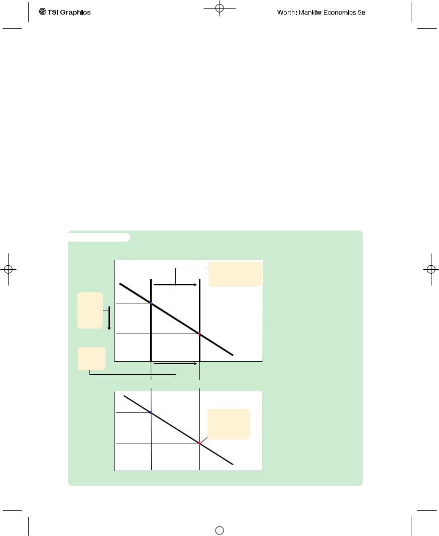
Figure 12-12 shows what happens when the price level falls. Because a lower price level raises the level of real money balances, the LM* curve shifts to the right, as in panel (a) of Figure 12-12.The real exchange rate depreciates, and the equilibrium level of income rises.The aggregate demand curve summarizes this negative relationship between the price level and the level of income, as shown in panel (b) of Figure 12-12.
Thus, just as the IS–LM model explains the aggregate demand curve in a closed economy, the Mundell–Fleming model explains the aggregate demand curve for a small open economy. In both cases, the aggregate demand curve shows the set of equilibria that arise as the price level varies. And in both cases, anything that changes the equilibrium for a given price level shifts the aggregate demand curve. Policies that raise income shift the aggregate demand curve to the right; policies that lower income shift the aggregate demand curve to the left.
f i g u r e 1 2 - 1 2
Real exchange rate, e
2. . . .
lowering e1 the real exchange
rate . . .
e2
3. . . . and raising income Y.
(a) The Mundell–Fleming Model
1. A fall in the price
LM*(P1) LM*(P2) level P shifts the LM* curve to the right, . . .
|
|
|
|
IS* |
|
|
|
Income, output, Y |
|
Y1 |
|
|
Y2 |
|
|
|
|||
|
|
|
|
|
(b) The Aggregate Demand Curve
Price level, P
P1 |
|
4. The AD curve |
||
|
|
|
|
summarizes the |
|
|
|
|
relationship |
|
|
|
|
between P and Y. |
P2 |
|
|
|
AD |
|
|
|||
|
|
|||
|
|
|
|
|
Y1 |
Y2 |
Income, output, Y |
||
Mundell–Fleming as a Theory
of Aggregate Demand Panel
(a)shows that when the price level falls, the LM* curve shifts to the right. The equilibrium level of income rises. Panel
(b)shows that this negative relationship between P and Y is summarized by the aggregate demand curve.
User JOEWA:Job EFF01428:6264_ch12:Pg 336:27531#/eps at 100% *27531* |
Mon, Feb 18, 2002 12:45 AM |
|||
|
|
|
|
|
|
|
|
|
|
C H A P T E R 1 2 Aggregate Demand in the Open Economy | 337
f i g u r e 1 2 - 1 3
(a) The Mundell–Fleming Model
Real exchange |
LM*(P1) |
LM*(P2) |
|
rate, e |
|
||
e1 |
K |
|
|
|
|
|
|
e2 |
|
C |
|
|
|
|
|
|
|
|
IS* |
|
Y1 |
Y |
Income, output, Y |
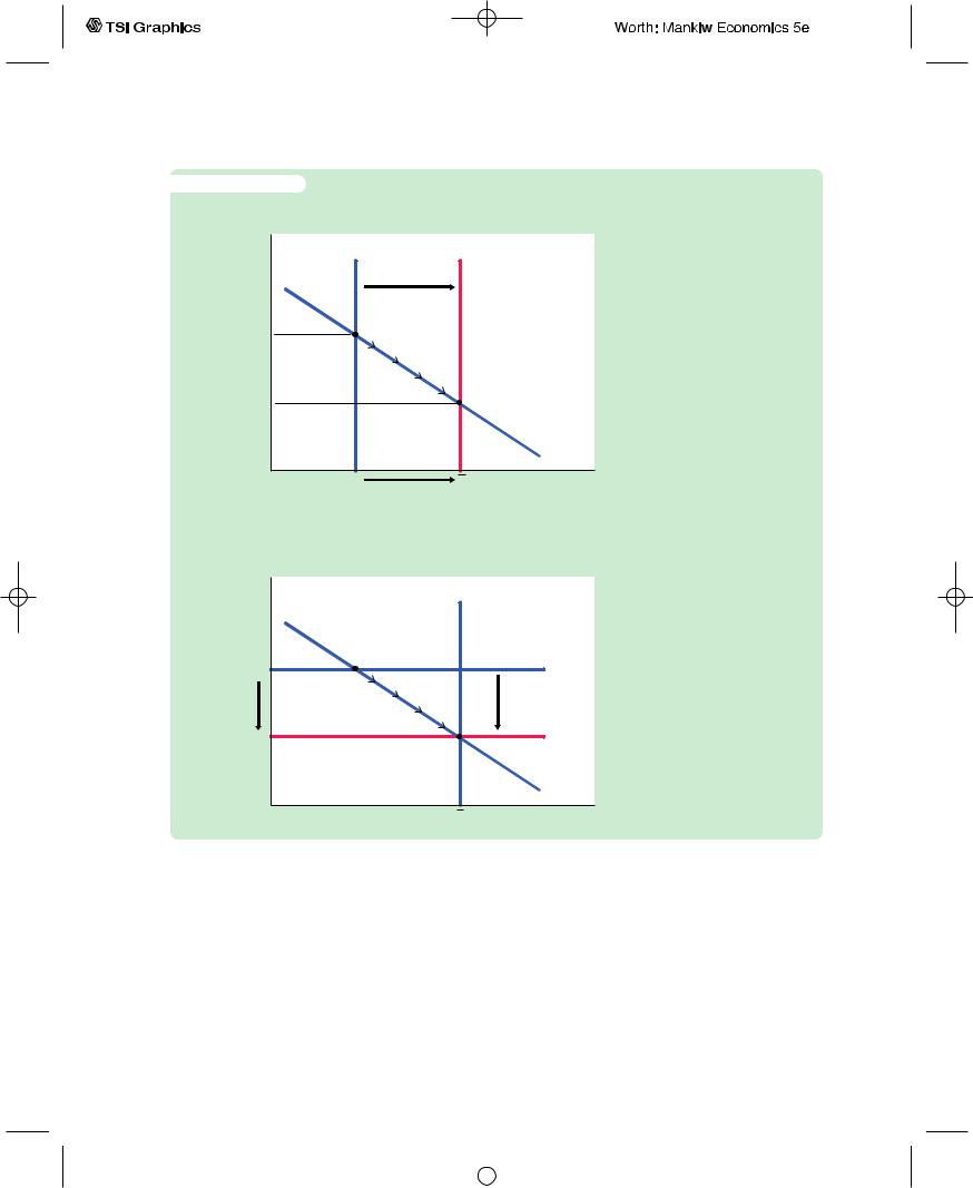
The Short-Run and Long-Run Equilibria in a Small Open Economy Point K in both panels shows the equilibrium under the Keynesian assumption that the price level is fixed at P1. Point C in both panels shows the equilibrium under the classical assumption that the price level
adjusts to maintain income at
−
its natural rate Y .
(b) The Model of Aggregate Supply
and Aggregate Demand
Price level, P
|
LRAS |
|
K |
P1 |
SRAS1 |
P2 |
SRAS2 |
|
C |
|
AD |
Y Income, output, Y
We can use this diagram to show how the short-run model in this chapter is related to the long-run model in Chapter 5. Figure 12-13 shows the short-run and long-run equilibria. In both panels of the figure, point K describes the short-run equilibrium, because it assumes a fixed price level.At this equilibrium, the demand for goods and services is too low to keep the economy producing at its natural rate. Over time, low demand causes the price level to fall.The fall in the price level raises real money balances, shifting the LM* curve to the right.The real exchange rate depreciates, so net exports rise. Eventually, the economy reaches point C, the longrun equilibrium. The speed of transition between the short-run and long-run equilibria depends on how quickly the price level adjusts to restore the economy to the natural rate.
User JOEWA:Job EFF01428:6264_ch12:Pg 337:27532#/eps at 100% *27532* |
Mon, Feb 18, 2002 12:45 AM |
|||
|
|
|
|
|
|
|
|
|
|

338 | P A R T I V Business Cycle Theory: The Economy in the Short Run
The levels of income at point K and point C are both of interest. Our central concern in this chapter has been how policy influences point K, the short-run equilibrium. In Chapter 5 we examined the determinants of point C, the longrun equilibrium. Whenever policymakers consider any change in policy, they need to consider both the short-run and long-run effects of their decision.
12-7 A Concluding Reminder
In this chapter we have examined how a small open economy works in the short run when prices are sticky.We have seen how monetary and fiscal policy influence income and the exchange rate, and how the behavior of the economy depends on whether the exchange rate is floating or fixed. In closing, it is worth repeating a lesson from Chapter 5. Many countries, including the United States, are neither closed economies nor small open economies: they lie somewhere in between.
A large open economy, such as the United States, combines the behavior of a closed economy and the behavior of a small open economy.When analyzing policies in a large open economy, we need to consider both the closed-economy logic of Chapter 11 and the open-economy logic developed in this chapter.The appendix to this chapter presents a model for a large open economy.The results of that model are, as one would guess, a mixture of the two polar cases we have already examined.
To see how we can draw on the logic of both the closed and small open economies and apply these insights to the United States, consider how a monetary contraction affects the economy in the short run. In a closed economy, a monetary contraction raises the interest rate, lowers investment, and thus lowers aggregate income. In a small open economy with a floating exchange rate, a monetary contraction raises the exchange rate, lowers net exports, and thus lowers aggregate income.The interest rate is unaffected, however, because it is determined by world financial markets.
The U.S. economy contains elements of both cases. Because the United States is large enough to affect the world interest rate and because capital is not perfectly mobile across countries, a monetary contraction does raise the interest rate and depress investment. At the same time, a monetary contraction also raises the value of the dollar, thereby depressing net exports. Hence, although the Mundell–Fleming model does not precisely describe an economy like that of the United States, it does predict correctly what happens to international variables such as the exchange rate, and it shows how international interactions alter the effects of monetary and fiscal policies.
Summary
1.The Mundell–Fleming model is the IS–LM model for a small open economy. It takes the price level as given and then shows what causes fluctuations in income and the exchange rate.
2.The Mundell–Fleming model shows that fiscal policy does not influence aggregate income under floating exchange rates. A fiscal expansion causes the
User JOEWA:Job EFF01428:6264_ch12:Pg 338:27533#/eps at 100% *27533* |
Mon, Feb 18, 2002 12:45 AM |
|||
|
|
|
|
|
|
|
|
|
|