Mankiw Macroeconomics (5th ed)

C H A P T E R 1 2 Aggregate Demand in the Open Economy | 319

Monetary Policy

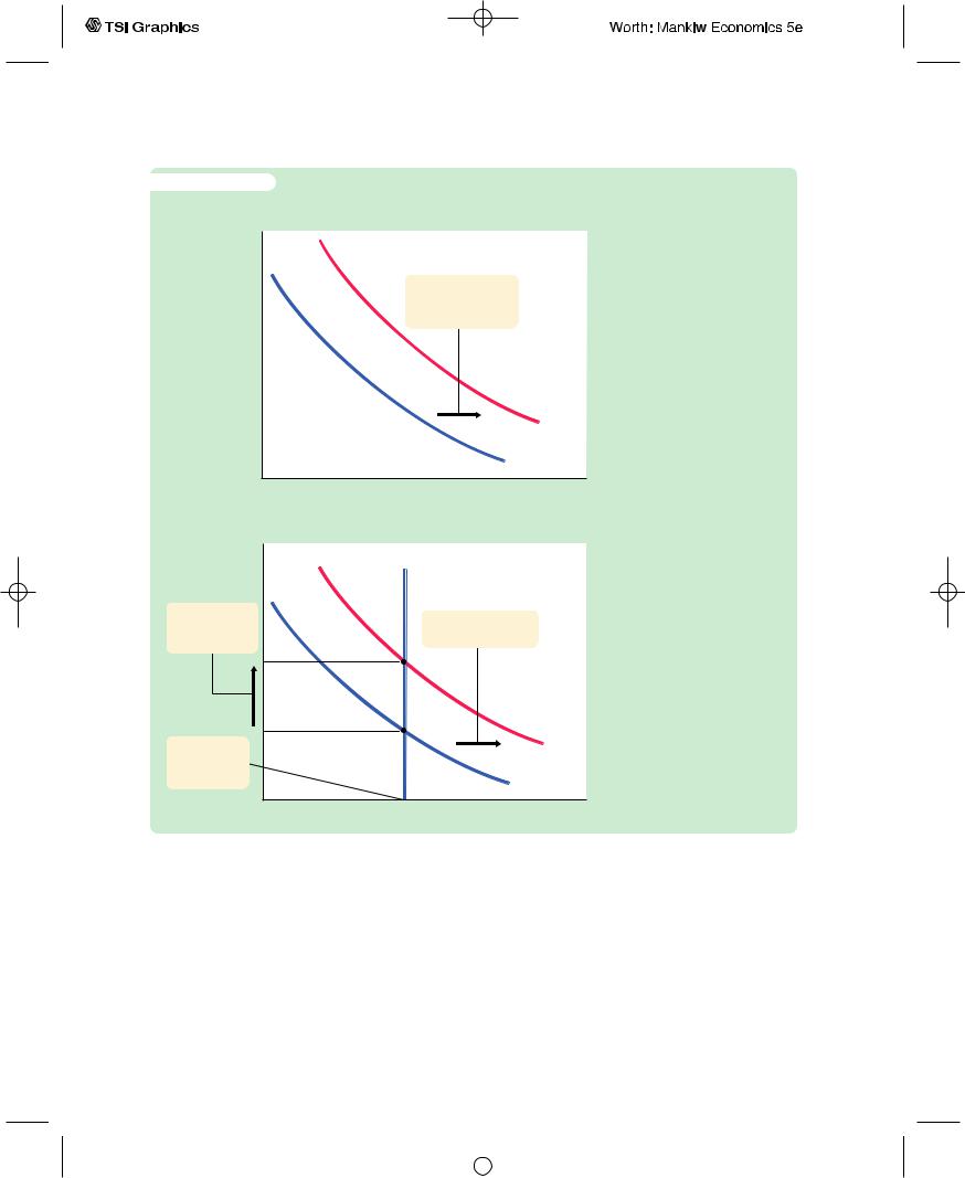
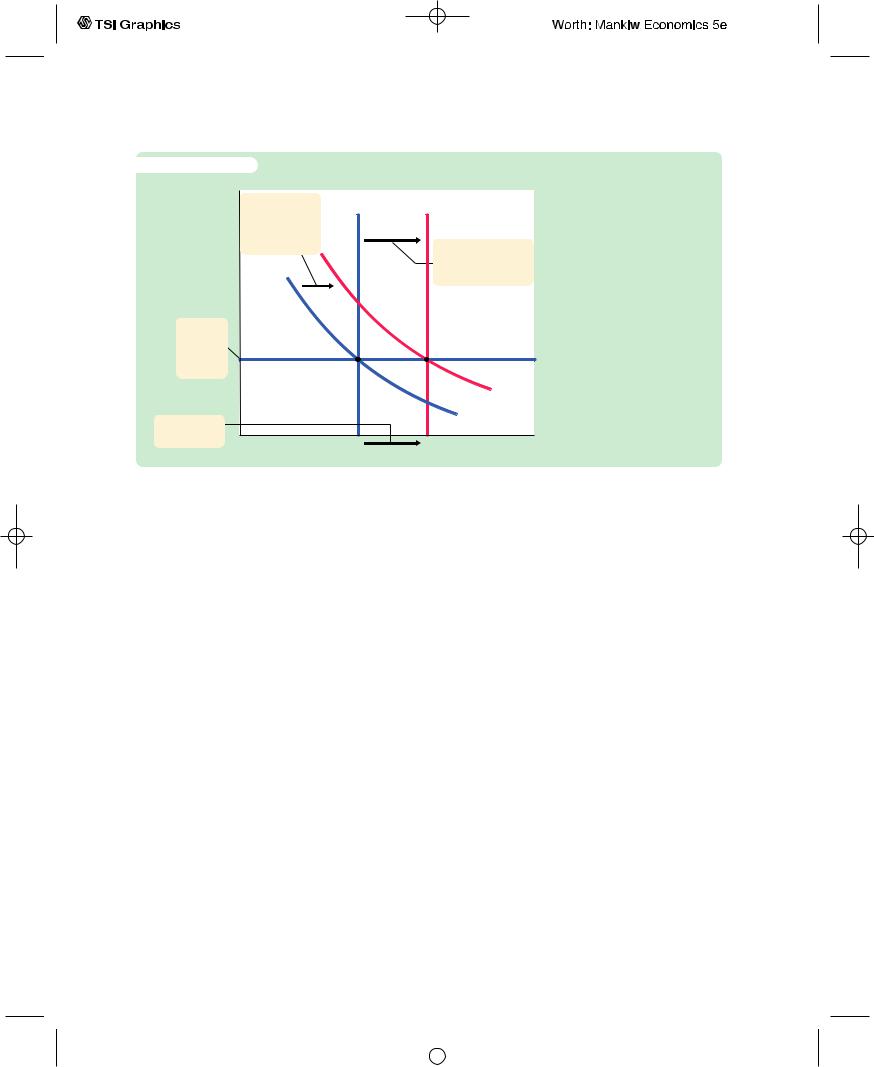
Suppose now that the central bank increases the money supply. Because the price level is assumed to be fixed, the increase in the money supply means an increase in real balances.The increase in real balances shifts the LM* curve to the right, as in Figure 12-5. Hence, an increase in the money supply raises income and lowers the exchange rate.

Income, output, Y

Although monetary policy influences income in an open economy, as it does in a closed economy, the monetary transmission mechanism is different. Recall that in a closed economy an increase in the money supply increases spending because it lowers the interest rate and stimulates investment. In a small open economy, the interest rate is fixed by the world interest rate. As soon as an increase in the money supply puts downward pressure on the domestic interest rate, capital flows out of the economy as investors seek a higher return elsewhere.This capital outflow prevents the domestic interest rate from falling. In addition, because the capital outflow increases the supply of the domestic currency in the market for foreign-currency exchange, the exchange rate depreciates. The fall in the exchange rate makes domestic goods inexpensive relative to foreign goods and, thereby, stimulates net exports. Hence, in a small open economy, monetary policy influences income by altering the exchange rate rather than the interest rate.

Trade Policy

Suppose that the government reduces the demand for imported goods by imposing an import quota or a tariff.What happens to aggregate income and the exchange rate?

Because net exports equal exports minus imports, a reduction in imports means an increase in net exports.That is, the net-exports schedule shifts to the

320 | P A R T I V Business Cycle Theory: The Economy in the Short Run

right, as in Figure 12-6. This shift in the net-exports schedule increases planned expenditure and thus moves the IS* curve to the right. Because the LM* curve is vertical, the trade restriction raises the exchange rate but does not affect income.

Often a stated goal of policies to restrict trade is to alter the trade balance NX. Yet, as we first saw in Chapter 5, such policies do not necessarily have that effect. The same conclusion holds in the Mundell–Fleming model under floating exchange rates. Recall that

NX(e) = Y − C(Y − T ) − I(r*) − G.

C H A P T E R 1 2 Aggregate Demand in the Open Economy | 321

Because a trade restriction does not affect income, consumption, investment, or government purchases, it does not affect the trade balance. Although the shift in the net-exports schedule tends to raise NX, the increase in the exchange rate reduces NX by the same amount.

12-3 The Small Open Economy Under Fixed

Exchange Rates

We now turn to the second type of exchange-rate system: fixed exchange rates. In the 1950s and 1960s, most of the world’s major economies, including the United States, operated within the Bretton Woods system—an international monetary system under which most governments agreed to fix exchange rates. The world abandoned this system in the early 1970s, and exchange rates were allowed to float. Some European countries later reinstated a system of fixed exchange rates among themselves, and some economists have advocated a return to a worldwide system of fixed exchange rates. In this section we discuss how such a system works, and we examine the impact of economic policies on an economy with a fixed exchange rate.

How a Fixed-Exchange-Rate System Works

Under a system of fixed exchange rates, a central bank stands ready to buy or sell the domestic currency for foreign currencies at a predetermined price. For example, suppose that the Fed announced that it was going to fix the exchange rate at 100 yen per dollar. It would then stand ready to give $1 in exchange for 100 yen or to give 100 yen in exchange for $1. To carry out this policy, the Fed would need a reserve of dollars (which it can print) and a reserve of yen (which it must have purchased previously).

A fixed exchange rate dedicates a country’s monetary policy to the single goal of keeping the exchange rate at the announced level. In other words, the essence of a fixed-exchange-rate system is the commitment of the central bank to allow the money supply to adjust to whatever level will ensure that the equilibrium exchange rate equals the announced exchange rate. Moreover, as long as the central bank stands ready to buy or sell foreign currency at the fixed exchange rate, the money supply adjusts automatically to the necessary level.

To see how fixing the exchange rate determines the money supply, consider the following example. Suppose that the Fed announces that it will fix the exchange rate at 100 yen per dollar, but, in the current equilibrium with the current money supply, the exchange rate is 150 yen per dollar. This situation is illustrated in panel (a) of Figure 12-7. Notice that there is a profit opportunity: an arbitrageur could buy 300 yen in the marketplace for $2, and then sell the yen to the Fed for $3, making a $1 profit.When the Fed buys these yen from the arbitrageur, the dollars it pays for them automatically increase the money supply. The

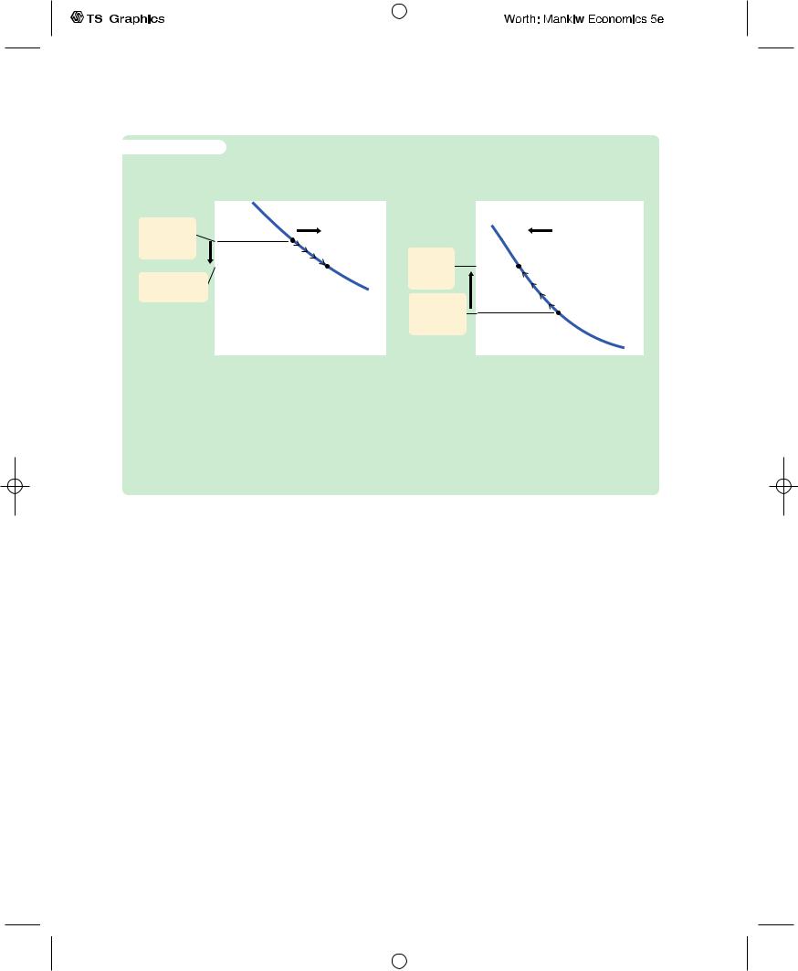
How a Fixed Exchange Rate Governs the Money Supply In panel (a), the equilibrium exchange rate initially exceeds the fixed level. Arbitrageurs will buy foreign currency in foreign-exchange markets and sell it to the Fed for a profit. This process automatically increases the money supply, shifting the LM* curve to the right and lowering the exchange rate. In panel (b), the equilibrium exchange rate is initially below the fixed level. Arbitrageurs will buy dollars in foreign-exchange markets and use them to buy foreign currency from the Fed. This process automatically reduces the money supply, shifting the LM* curve to the left and raising the exchange rate.

rise in the money supply shifts the LM* curve to the right, lowering the equilibrium exchange rate. In this way, the money supply continues to rise until the equilibrium exchange rate falls to the announced level.

Conversely, suppose that when the Fed announces that it will fix the exchange rate at 100 yen per dollar, the equilibrium is 50 yen per dollar. Panel (b) of Figure 12-7 shows this situation. In this case, an arbitrageur could make a profit by buying 100 yen from the Fed for $1 and then selling the yen in the marketplace for $2. When the Fed sells these yen, the $1 it receives automatically reduces the money supply. The fall in the money supply shifts the LM* curve to the left, raising the equilibrium exchange rate. The money supply continues to fall until the equilibrium exchange rate rises to the announced level.

It is important to understand that this exchange-rate system fixes the nominal exchange rate. Whether it also fixes the real exchange rate depends on the time horizon under consideration. If prices are flexible, as they are in the long run, then the real exchange rate can change even while the nominal exchange rate is fixed. Therefore, in the long run described in Chapter 5, a policy to fix the nominal exchange rate would not influence any real variable, including the real exchange rate. A fixed nominal exchange rate would influence only the money supply and the price level.Yet in the short run described by the Mundell–Fleming model, prices are fixed, so a fixed nominal exchange rate implies a fixed real exchange rate as well.

C H A P T E R 1 2 Aggregate Demand in the Open Economy | 323

C A S E S T U D Y

The International Gold Standard

During the late nineteenth and early twentieth centuries, most of the world’s major economies operated under a gold standard. Each country maintained a reserve of gold and agreed to exchange one unit of its currency for a specified amount of gold.Through the gold standard, the world’s economies maintained a system of fixed exchange rates.

To see how an international gold standard fixes exchange rates, suppose that the U.S. Treasury stands ready to buy or sell 1 ounce of gold for $100, and the Bank of England stands ready to buy or sell 1 ounce of gold for 100 pounds.Together, these policies fix the rate of exchange between dollars and pounds: $1 must trade for 1 pound. Otherwise, the law of one price would be violated, and it would be profitable to buy gold in one country and sell it in the other.

For example, suppose that the exchange rate were 2 pounds per dollar. In this case, an arbitrageur could buy 200 pounds for $100, use the pounds to buy 2 ounces of gold from the Bank of England, bring the gold to the United States, and sell it to the Treasury for $200—making a $100 profit. Moreover, by bringing the gold to the United States from England, the arbitrageur would increase the money supply in the United States and decrease the money supply in England.

Thus, during the era of the gold standard, the international transport of gold by arbitrageurs was an automatic mechanism adjusting the money supply and stabilizing exchange rates. This system did not completely fix exchange rates, because shipping gold across the Atlantic was costly.Yet the international gold standard did keep the exchange rate within a range dictated by transportation costs. It thereby prevented large and persistent movements in exchange rates.2

Fiscal Policy

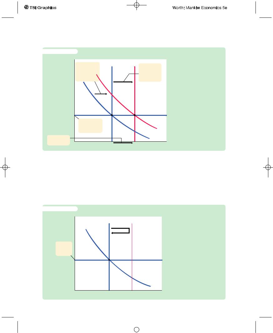
Let’s now examine how economic policies affect a small open economy with a fixed exchange rate. Suppose that the government stimulates domestic spending by increasing government purchases or by cutting taxes.This policy shifts the IS* curve to the right, as in Figure 12-8, putting upward pressure on the exchange rate. But because the central bank stands ready to trade foreign and domestic currency at the fixed exchange rate, arbitrageurs quickly respond to the rising exchange rate by selling foreign currency to the central bank, leading to an automatic monetary expansion. The rise in the money supply shifts the LM* curve to the right.Thus, under a fixed exchange rate, a fiscal expansion raises aggregate income.

2 For more on how the gold standard worked, see the essays in Barry Eichengreen, ed., The Gold Standard in Theory and History (NewYork: Methuen, 1985).

324 | P A R T I V Business Cycle Theory: The Economy in the Short Run

Monetary Policy

Imagine that a central bank operating with a fixed exchange rate were to try to increase the money supply—for example, by buying bonds from the public.What would happen? The initial impact of this policy is to shift the LM* curve to the right, lowering the exchange rate, as in Figure 12-9. But, because the central bank is committed to trading foreign and domestic currency at a fixed exchange

C H A P T E R 1 2 Aggregate Demand in the Open Economy | 325

rate, arbitrageurs quickly respond to the falling exchange rate by selling the domestic currency to the central bank, causing the money supply and the LM* curve to return to their initial positions. Hence, monetary policy as usually conducted is ineffectual under a fixed exchange rate. By agreeing to fix the exchange rate, the central bank gives up its control over the money supply.

A country with a fixed exchange rate can, however, conduct a type of monetary policy: it can decide to change the level at which the exchange rate is fixed. A reduction in the value of the currency is called a devaluation, and an increase in its value is called a revaluation. In the Mundell–Fleming model, a devaluation shifts the LM* curve to the right; it acts like an increase in the money supply under a floating exchange rate. A devaluation thus expands net exports and raises aggregate income. Conversely, a revaluation shifts the LM* curve to the left, reduces net exports, and lowers aggregate income.

C A S E S T U D Y

Devaluation and the Recovery From the Great Depression

The Great Depression of the 1930s was a global problem.Although events in the United States may have precipitated the downturn, all of the world’s major economies experienced huge declines in production and employment.Yet not all governments responded to this calamity in the same way.

One key difference among governments was how committed they were to the fixed exchange rate set by the international gold standard. Some countries, such as France, Germany, Italy, and the Netherlands, maintained the old rate of exchange between gold and currency. Other countries, such as Denmark, Finland, Norway, Sweden, and the United Kingdom, reduced the amount of gold they would pay for each unit of currency by about 50 percent. By reducing the gold content of their currencies, these governments devalued their currencies relative to those of other countries.

The subsequent experience of these two groups of countries conforms to the prediction of the Mundell–Fleming model.Those countries that pursued a policy of devaluation recovered quickly from the Depression.The lower value of the currency raised the money supply, stimulated exports, and expanded production. By contrast, those countries that maintained the old exchange rate suffered longer with a depressed level of economic activity.3

Trade Policy

Suppose that the government reduces imports by imposing an import quota or a tariff.This policy shifts the net-exports schedule to the right and thus shifts the IS* curve to the right, as in Figure 12-10. The shift in the IS* curve tends to

3 Barry Eichengreen and Jeffrey Sachs, “Exchange Rates and Economic Recovery in the 1930s,”

Journal of Economic History 45 (December 1985): 925–946.

326 | P A R T I V Business Cycle Theory: The Economy in the Short Run

raise the exchange rate.To keep the exchange rate at the fixed level, the money supply must rise, shifting the LM* curve to the right.

The result of a trade restriction under a fixed exchange rate is very different from that under a floating exchange rate. In both cases, a trade restriction shifts the net-exports schedule to the right, but only under a fixed exchange rate does a trade restriction increase net exports NX.The reason is that a trade restriction under a fixed exchange rate induces monetary expansion rather than an appreciation of the exchange rate.The monetary expansion, in turn, raises aggregate income. Recall the accounting identity

NX = S − I.

When income rises, saving also rises, and this implies an increase in net exports.

Policy in the Mundell–Fleming Model: A Summary

The Mundell–Fleming model shows that the effect of almost any economic policy on a small open economy depends on whether the exchange rate is floating or fixed. Table 12-1 summarizes our analysis of the short-run effects of fiscal, monetary, and trade policies on income, the exchange rate, and the trade balance. What is most striking is that all of the results are different under floating and fixed exchange rates.

To be more specific, the Mundell–Fleming model shows that the power of monetary and fiscal policy to influence aggregate income depends on the exchange-rate regime. Under floating exchange rates, only monetary policy can affect income.The usual expansionary impact of fiscal policy is offset by a rise in

C H A P T E R 1 2 Aggregate Demand in the Open Economy | 327

t a b l e 1 2 - 1

The Mundell–Fleming Model: Summary of Policy Effects

Note: This table shows the direction of impact of various economic policies on income Y, the exchange rate e, and the trade balance NX. A “↑” indicates that the variable increases; a “↓” indicates that it decreases; a “0’’ indicates no effect. Remember that the exchange rate is defined as the amount of foreign currency per unit of domestic currency (for example, 100 yen per dollar).

the value of the currency. Under fixed exchange rates, only fiscal policy can affect income.The normal potency of monetary policy is lost because the money supply is dedicated to maintaining the exchange rate at the announced level.

12-4 Interest-Rate Differentials

So far, our analysis has assumed that the interest rate in a small open economy is equal to the world interest rate: r = r*.To some extent, however, interest rates differ around the world.We now extend our analysis by considering the causes and effects of international interest-rate differentials.

Country Risk and Exchange-Rate Expectations

When we assumed earlier that the interest rate in our small open economy is determined by the world interest rate, we were applying the law of one price.We reasoned that if the domestic interest rate were above the world interest rate, people from abroad would lend to that country, driving the domestic interest rate down. And if the domestic interest rate were below the world interest rate, domestic residents would lend abroad to earn a higher return, driving the domestic interest rate up. In the end, the domestic interest rate would equal the world interest rate.

Why doesn’t this logic always apply? There are two reasons.

One reason is country risk. When investors buy U.S. government bonds or make loans to U.S. corporations, they are fairly confident that they will be repaid with interest. By contrast, in some less developed countries, it is plausible to fear that a revolution or other political upheaval might lead to a default on loan repayments. Borrowers in such countries often have to pay higher interest rates to compensate lenders for this risk.

328 | P A R T I V Business Cycle Theory: The Economy in the Short Run

Another reason interest rates differ across countries is expected changes in the exchange rate. For example, suppose that people expect the French franc to fall in value relative to the U.S. dollar.Then loans made in francs will be repaid in a less valuable currency than loans made in dollars. To compensate for this expected fall in the French currency, the interest rate in France will be higher than the interest rate in the United States.

Thus, because of both country risk and expectations of future exchange-rate changes, the interest rate of a small open economy can differ from interest rates in other economies around the world. Let’s now see how this fact affects our analysis.

Differentials in the Mundell–Fleming Model

To incorporate interest-rate differentials into the Mundell–Fleming model, we assume that the interest rate in our small open economy is determined by the world interest rate plus a risk premium v:

r = r* + v.

The risk premium is determined by the perceived political risk of making loans in a country and the expected change in the real exchange rate. For our purposes here, we can take the risk premium as exogenous in order to examine how changes in the risk premium affect the economy.

The model is largely the same as before.The two equations are

For any given fiscal policy, monetary policy, price level, and risk premium, these two equations determine the level of income and exchange rate that equilibrate the goods market and the money market. Holding constant the risk premium, the tools of monetary, fiscal, and trade policy work as we have already seen.

Now suppose that political turmoil causes the country’s risk premium v to rise.The most direct effect is that the domestic interest rate r rises.The higher interest rate, in turn, has two effects. First, the IS* curve shifts to the left, because the higher interest rate reduces investment. Second, the LM* curve shifts to the right, because the higher interest rate reduces the demand for money, and this allows a higher level of income for any given money supply. [Recall that Y must satisfy the equation M/P = L(r* + v, Y ).] As Figure 12-11 shows, these two shifts cause income to rise and the currency to depreciate.

This analysis has an important implication: expectations of the exchange rate are partially self-fulfilling. For example, suppose that people come to believe that the French franc will not be valuable in the future. Investors will place a larger risk premium on French assets: v will rise in France.This expectation will drive