

Mankiw Macroeconomics (5th ed)
.pdfC H A P T E R 1 1 Aggregate Demand II | 309
This equation simply equates money supply and money demand.
We can learn more about the LM curve by considering the case in which the money demand function is linear—that is,
L(r, Y ) = eY − fr,
where e and f are numbers greater than zero. The value of e determines how much the demand for money rises when income rises.The value of f determines how much the demand for money falls when the interest rate rises. There is a minus sign in front of the interest rate term because money demand is inversely related to the interest rate.
The equilibrium in the money market is now described by
M/P = eY − fr.
To see what this equation implies, rearrange the terms so that r is on the lefthand side.We obtain
r = (e/f )Y − (1/f )M/P.
This equation gives us the interest rate that equilibrates the money market for any values of income and real money balances.The LM curve graphs this equation for different values of Y and r given a fixed value of M/P.
From this last equation, we can verify some of our conclusions about the LM curve. First, because the coefficient of income is positive, the LM curve slopes upward: higher income requires a higher interest rate to equilibrate the money market. Second, because the coefficient of real money balances is negative, decreases in real balances shift the LM curve upward, and increases in real balances shift the LM curve downward.
From the coefficient of income, e/f, we can see what determines whether the LM curve is steep or flat. If money demand is not very sensitive to the level of income, then e is small. In this case, only a small change in the interest rate is necessary to offset the small increase in money demand caused by a change in income: the LM curve is relatively flat. Similarly, if the quantity of money demanded is not very sensitive to the interest rate, then f is small. In this case, a shift in money demand caused by a change in income leads to a large change in the equilibrium interest rate: the LM curve is relatively steep.
The Aggregate Demand Curve
To find the aggregate demand equation, we must find the level of income that satisfies both the IS equation and the LM equation.To do this, substitute the LM equation for the interest rate r into the IS equation to obtain
a + c |
1 |
|
−b |
|
−d |
Y = + G + T + |
|||||
1 − b 1 |
− b |
1 |
− b |
1 |
− b |
e |
1 |
M |
). |
( f |
Y − f |
P |
User JOEWA:Job EFF01427:6264_ch11:Pg 309:27356#/eps at 100% *27356* |
Wed, Feb 13, 2002 10:28 AM |
|||
|
|
|
|
|
|
|
|
|
|

310 | P A R T I V Business Cycle Theory: The Economy in the Short Run
With some algebraic manipulation, we can solve for Y. The final equation for Y is
z(a + c) |
|
z |
−zb |
|
d |
M |
Y = + G + T + , |
||||||
1 − b |
1 |
− b |
1 − b |
(1 |
− b)[f + de/(1 |
− b)] P |
where z = f/[f + de/(1 − b)] is a composite of some of the parameters and is between zero and one.
This last equation expresses the aggregate demand curve algebraically. It says that income depends on fiscal policy G and T, monetary policy M, and the price level P. The aggregate demand curve graphs this equation for different values of Y and P given fixed values of G, T, and M.
We can explain the slope and position of the aggregate demand curve with this equation. First, the aggregate demand curve slopes downward, because an increase in P lowers M/P and thus lowers Y. Second, increases in the money supply raise income and shift the aggregate demand curve to the right. Third, increases in government purchases or decreases in taxes also raise income and shift the aggregate demand curve to the right. Note that, because z is less than one, the multipliers for fiscal policy are smaller in the IS–LM model than in the Keynesian cross. Hence, the parameter z reflects the crowding out of investment discussed earlier.
Finally, this equation shows the relationship between the aggregate demand curve derived in this chapter from the IS–LM model and the aggregate demand curve derived in Chapter 9 from the quantity theory of money. The quantity theory assumes that the interest rate does not influence the quantity of real money balances demanded. Put differently, the quantity theory assumes that the parameter f equals zero. If f equals zero, then the composite parameter z also equals zero, so fiscal policy does not influence aggregate demand. Thus, the aggregate demand curve derived in Chapter 9 is a special case of the aggregate demand curve derived here.
C A S E S T U D Y
The Effectiveness of Monetary and Fiscal Policy
Economists have long debated whether monetary or fiscal policy exerts a more powerful influence on aggregate demand. According to the IS–LM model, the answer to this question depends on the parameters of the IS and LM curves. Therefore, economists have spent much energy arguing about the size of these parameters.The most hotly contested parameters are those that describe the influence of the interest rate on economic decisions.
Those economists who believe that fiscal policy is more potent than monetary policy argue that the responsiveness of investment to the interest rate— measured by the parameter d—is small. If you look at the algebraic equation for aggregate demand, you will see that a small value of d implies a small effect of the money supply on income. The reason is that when d is small, the IS curve is nearly vertical, and shifts in the LM curve do not cause much of a
User JOEWA:Job EFF01427:6264_ch11:Pg 310:27357#/eps at 100% *27357* |
Wed, Feb 13, 2002 10:28 AM |
|||
|
|
|
|
|
|
|
|
|
|
C H A P T E R 1 1 Aggregate Demand II | 311
change in income. In addition, a small value of d implies a large value of z, which in turn implies that fiscal policy has a large effect on income.The reason for this large effect is that when investment is not very responsive to the interest rate, there is little crowding out.
Those economists who believe that monetary policy is more potent than fiscal policy argue that the responsiveness of money demand to the interest rate— measured by the parameter f—is small.When f is small, z is small, and fiscal policy has a small effect on income; in this case, the LM curve is nearly vertical. In addition, when f is small, changes in the money supply have a large effect on income.
Few economists today endorse either of these extreme views. The evidence indicates that the interest rate affects both investment and money demand. This finding implies that both monetary and fiscal policy are important determinants of aggregate demand.
M O R E P R O B L E M S A N D A P P L I C A T I O N S
1.Give an algebraic answer to each of the following questions. Then explain in words the economics that underlies your answer.
a.How does the sensitivity of investment to the interest rate affect the slope of the aggregate demand curve?
b.How does the sensitivity of money demand to the interest rate affect the slope of the aggregate demand curve?
c.How does the marginal propensity to consume affect the response of aggregate demand to changes in government purchases?
User JOEWA:Job EFF01427:6264_ch11:Pg 311:27358#/eps at 100% *27358* |
Wed, Feb 13, 2002 10:28 AM |
|||
|
|
|
|
|
|
|
|
|
|

C H A P T1E R 2 T W E L V E
Aggregate Demand in the
Open Economy
When conducting monetary and fiscal policy, policymakers often look beyond their own country’s borders. Even if domestic prosperity is their sole objective, it is necessary for them to consider the rest of the world. The international flow of goods and services and the international flow of capital can affect an economy in profound ways. Policymakers ignore these effects at their peril.
In this chapter we extend our analysis of aggregate demand to include international trade and finance. The model developed in this chapter, called the Mundell–Fleming model, is an open-economy version of the IS–LM model. Both models stress the interaction between the goods market and the money market. Both models assume that the price level is fixed and then show what causes short-run fluctuations in aggregate income (or, equivalently, shifts in the aggregate demand curve).The key difference is that the IS–LM model assumes a closed economy, whereas the Mundell–Fleming model assumes an open economy.The Mundell–Fleming model extends the short-run model of national income from Chapters 10 and 11 by including the effects of international trade and finance from Chapter 5.
The Mundell–Fleming model makes one important and extreme assumption: it assumes that the economy being studied is a small open economy with perfect capital mobility.That is, the economy can borrow or lend as much as it wants in world financial markets and, as a result, the economy’s interest rate is determined by the world interest rate. One virtue of this assumption is that it simplifies the analysis: once the interest rate is determined, we can concentrate our attention on the role of the exchange rate. In addition, for some economies, such as Belgium or the Netherlands, the assumption of a small open economy with perfect capital mobility is a good one. Yet this assump- tion—and thus the Mundell–Fleming model—does not apply exactly to a large open economy such as the United States. In the conclusion to this chapter (and more fully in the appendix), we consider what happens in the more complex case in which international capital mobility is less than perfect or a nation is so large it can influence world financial markets.
One lesson from the Mundell–Fleming model is that the behavior of an economy depends on the exchange-rate system it has adopted.We begin by assuming that the economy operates with a floating exchange rate.That is, we assume that the central bank allows the exchange rate to adjust to changing economic conditions.We then examine how the economy operates under a fixed exchange rate,
312 |
User JOEWA:Job EFF01428:6264_ch12:Pg 312:25875#/eps at 100% *25875* |
Mon, Feb 18, 2002 12:44 AM |
|||
|
|
|
|
|
|
|
|
|
|

C H A P T E R 1 2 Aggregate Demand in the Open Economy | 313
and we discuss whether a floating or fixed exchange rate is better.This question has been important in recent years, as many nations around the world have debated what exchange-rate system to adopt.
12-1 The Mundell–Fleming Model
In this section we build the Mundell–Fleming model, and in the following sections we use the model to examine the impact of various policies. As you will see, the Mundell–Fleming model is built from components we have used in previous chapters. But these pieces are put together in a new way to address a new set of questions.1
The Key Assumption: Small Open Economy With
Perfect Capital Mobility
Let’s begin with the assumption of a small open economy with perfect capital mobility. As we saw in Chapter 5, this assumption means that the interest rate in this economy r is determined by the world interest rate r*. Mathematically, we can write this assumption as
r = r*.
This world interest rate is assumed to be exogenously fixed because the economy is sufficiently small relative to the world economy that it can borrow or lend as much as it wants in world financial markets without affecting the world interest rate.
Although the idea of perfect capital mobility is expressed with a simple equation, it is important not to lose sight of the sophisticated process that this equation represents. Imagine that some event were to occur that would normally raise the interest rate (such as a decline in domestic saving). In a small open economy, the domestic interest rate might rise by a little bit for a short time, but as soon as it did, foreigners would see the higher interest rate and start lending to this country (by, for instance, buying this country’s bonds).The capital inflow would drive the domestic interest rate back toward r*. Similarly, if any event were ever to start driving the domestic interest rate downward, capital would flow out of the country to earn a higher return abroad, and this capital outflow would drive the domestic interest rate back upward toward r*. Hence, the r = r* equation represents the assumption that the international flow of capital is rapid enough to keep the domestic interest rate equal to the world interest rate.
1 The Mundell–Fleming model was developed in the early 1960s. Mundell’s contributions are collected in Robert A. Mundell, International Economics (New York: Macmillan, 1968). For Fleming’s contribution, see J. Marcus Fleming,“Domestic Financial Policies Under Fixed and Under Floating Exchange Rates,’’ IMF Staff Papers 9 (November 1962): 369–379. In 1999, Robert Mundell was awarded the Nobel Prize for his work in open-economy macroeconomics.
User JOEWA:Job EFF01428:6264_ch12:Pg 313:27508#/eps at 100% *27508* |
Mon, Feb 18, 2002 12:44 AM |
|||
|
|
|
|
|
|
|
|
|
|

314 | P A R T I V Business Cycle Theory: The Economy in the Short Run
The Goods Market and the IS* Curve
The Mundell–Fleming model describes the market for goods and services much as the IS–LM model does, but it adds a new term for net exports. In particular, the goods market is represented with the following equation:
Y = C(Y − T ) + I(r*) + G + NX(e).
This equation states that aggregate income Y is the sum of consumption C, investment I, government purchases G, and net exports NX. Consumption depends positively on disposable income Y − T. Investment depends negatively on the interest rate, which equals the world interest rate r*. Net exports depend negatively on the exchange rate e.As before, we define the exchange rate e as the amount of foreign currency per unit of domestic currency—for example, e might be 100 yen per dollar.
You may recall that in Chapter 5 we related net exports to the real exchange rate (the relative price of goods at home and abroad) rather than the nominal exchange rate (the relative price of domestic and foreign currencies). If e is the nominal exchange rate, then the real exchange rate e equals eP/P*, where P is the domestic price level and P* is the foreign price level.The Mundell–Fleming model, however, assumes that the price levels at home and abroad are fixed, so the real exchange rate is proportional to the nominal exchange rate. That is, when the nominal exchange rate appreciates (say, from 100 to 120 yen per dollar), foreign goods become cheaper compared to domestic goods, and this causes exports to fall and imports to rise.
We can illustrate this equation for goods market equilibrium on a graph in which income is on the horizontal axis and the exchange rate is on the vertical axis.This curve is shown in panel (c) of Figure 12-1 and is called the IS* curve. The new label reminds us that the curve is drawn holding the interest rate constant at the world interest rate r*.
The IS* curve slopes downward because a higher exchange rate reduces net exports, which in turn lowers aggregate income. To show how this works, the other panels of Figure 12-1 combine the net-exports schedule and the Keynesian cross to derive the IS* curve. In panel (a), an increase in the exchange rate from e1 to e2 lowers net exports from NX(e1) to NX(e2). In panel (b), the reduction in net exports shifts the planned-expenditure schedule downward and thus lowers income from Y1 to Y2. The IS* curves summarizes this relationship between the exchange rate e and income Y.
The Money Market and the LM* Curve
The Mundell–Fleming model represents the money market with an equation that should be familiar from the IS–LM model, with the additional assumption that the domestic interest rate equals the world interest rate:
M/P = L(r*, Y ).
User JOEWA:Job EFF01428:6264_ch12:Pg 314:27509#/eps at 100% *27509* |
Mon, Feb 18, 2002 12:44 AM |
|||
|
|
|
|
|
|
|
|
|
|
C H A P T E R 1 2 Aggregate Demand in the Open Economy | 315
f i g u r e 1 2 - 1
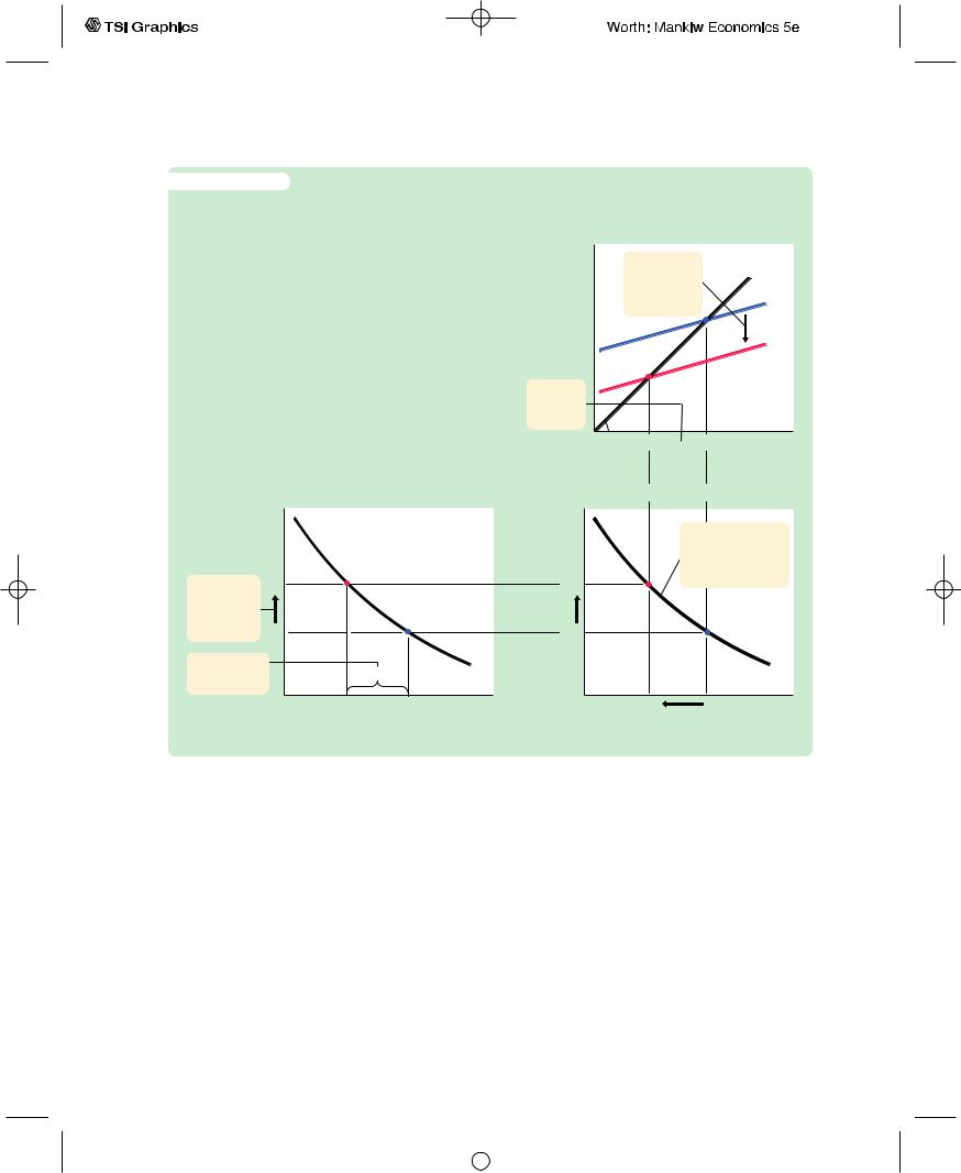
The IS* Curve The IS* curve is derived from the net-exports schedule and the Keynesian cross. Panel (a) shows the net-exports schedule: an increase in the exchange rate from e1 to e2 lowers net exports from NX(e1) to NX(e2). Panel (b) shows the Keynesian cross: a decrease in net exports from NX(e1) to NX(e2) shifts the plannedexpenditure schedule downward and reduces income from Y1 to Y2. Panel (c) shows the IS* curve summarizing this relationship between the exchange rate and income: the higher the exchange rate, the lower the level of income.
(b) The Keynesian Cross
Expenditure, E
3. . . . which shifts planned expenditure downward . . .
4. . . . and lowers income.
Y2  Y1
Y1
Actual expenditure
NX
Income, output, Y
(a) The Net-Exports Schedule
Exchange rate, e
1. An |
e2 |
increase in |
|
the exchange |
|
rate . .. |
e1 |
2. . . . lowers net exports, . . .
NX
NX(e2)  NX(e1) Net exports,
NX
Exchange rate, e
e2
e1
(c)The IS* Curve
5.The IS* curve summarizes these changes in the goods market equilibrium.
|
|
IS* |
Y2 |
Y1 |
Income, |
|
|
output, Y |
This equation states that the supply of real money balances, M/P, equals the demand, L(r, Y ). The demand for real balances depends negatively on the interest rate, which is now set equal to the world interest rate r*, and positively on income Y. The money supply M is an exogenous variable controlled by the central bank, and because the Mundell–Fleming model is designed to analyze short-run fluctuations, the price level P is also assumed to be exogenously fixed.
We can represent this equation graphically with a vertical LM* curve, as in panel (b) of Figure 12-2. The LM* curve is vertical because the exchange rate does not enter into the LM* equation. Given the world interest rate, the LM* equation determines aggregate income, regardless of the exchange rate. Figure 12-2 shows how the LM* curve arises from the world interest rate and the LM curve, which relates the interest rate and income.
User JOEWA:Job EFF01428:6264_ch12:Pg 315:27510#/eps at 100% *27510* |
Mon, Feb 18, 2002 12:44 AM |
|||
|
|
|
|
|
|
|
|
|
|
316 | P A R T I V Business Cycle Theory: The Economy in the Short Run
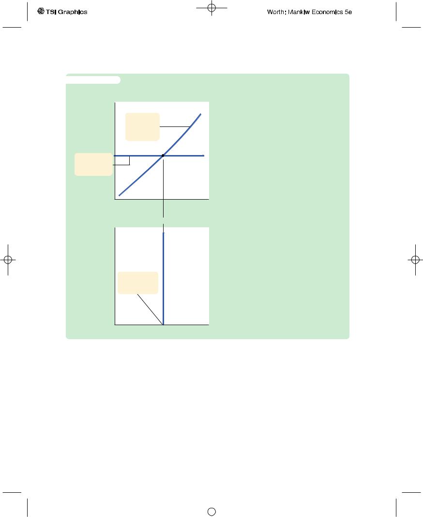
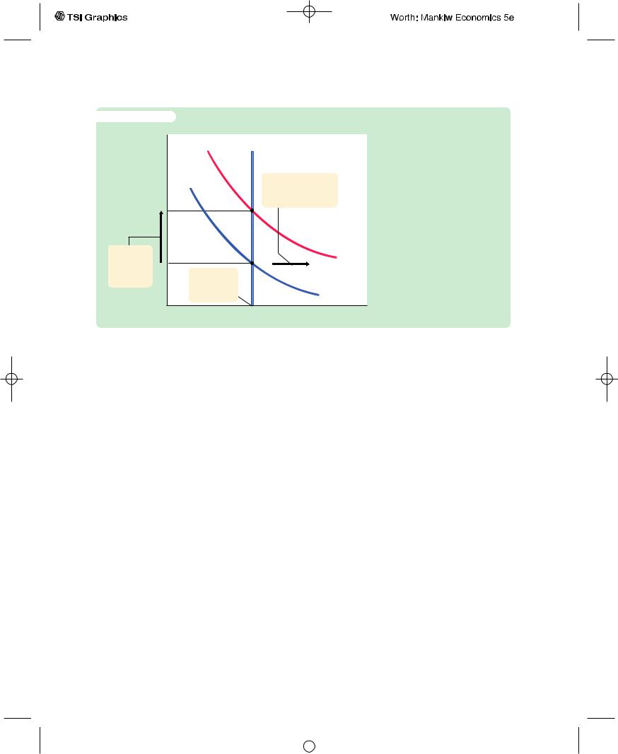
f i g u r e 1 2 - 2
(a) The LM Curve
Interest rate, r
LM
1. The money market equilibrium condition . . .
r r*
2. . . . and the world
interest rate . . .
The LM* Curve Panel (a) shows the standard LM curve [which graphs the equation M/P = L(r, Y )] together with a horizontal line representing the world interest rate r*. The intersection of these two curves determines the level of income, regardless of the exchange rate. Therefore, as panel (b) shows, the LM* curve is vertical.
Income, output, Y
(b) The LM* Curve
Exchange rate, e
LM*
3. . . . determine the level of income.
Income, output, Y
Putting the Pieces Together
According to the Mundell–Fleming model, a small open economy with perfect capital mobility can be described by two equations:
Y = C(Y − T ) + I(r*) + G + NX(e) |
IS*, |
M/P = L(r*, Y ) |
LM*. |
The first equation describes equilibrium in the goods market, and the second equation describes equilibrium in the money market. The exogenous variables are fiscal policy G and T, monetary policy M, the price level P, and the world interest rate r*.The endogenous variables are income Y and the exchange rate e.
Figure 12-3 illustrates these two relationships.The equilibrium for the economy is found where the IS* curve and the LM* curve intersect.This intersection
User JOEWA:Job EFF01428:6264_ch12:Pg 316:27511#/eps at 100% *27511* |
Mon, Feb 18, 2002 12:44 AM |
|||
|
|
|
|
|
|
|
|
|
|
|
|
|
|
|
|
|
|
|
|
|
|
|
|
|
1 2 Aggregate Demand in the Open Economy | 317 |
||
|
|
|
|
|
|
|||
|
|
C H A P T E R |
||||||
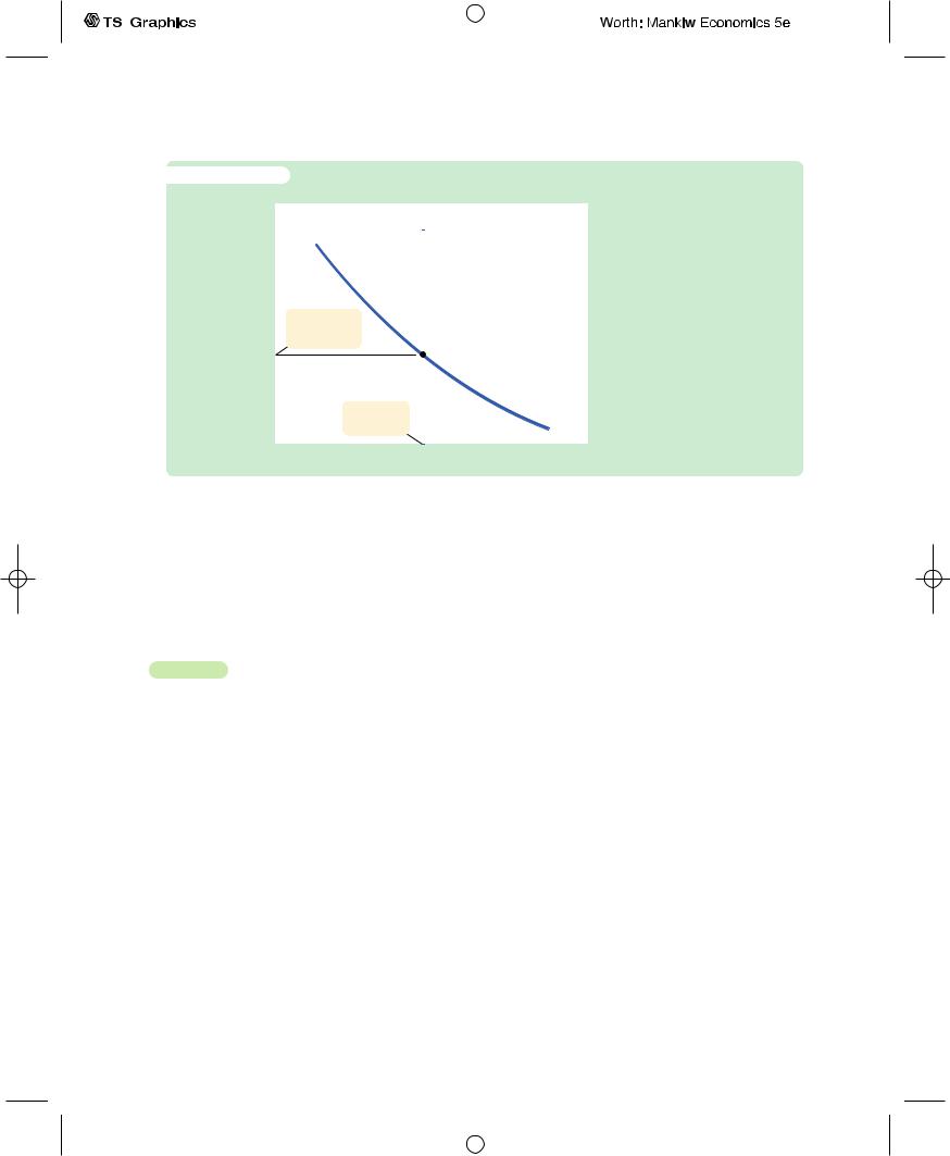
f i g u r e 1 2 - 3 |
|
|
|
|||||
Exchange rate, e |
|
|
|
|
|
The Mundell–Fleming Model |
||
|
||||||||
|
|
LM* |
|
|
This graph of the Mundell– |
|||
|
|
|
|
|
|
|
|
Fleming model plots the |
|
|
|
|
|
|
|
|
goods market equilibrium |
|
|
|
|
|
|
|
|
condition IS* and the money |
|
|
|
|
|
|
|
|
market equilibrium condition |
|
|
|
|
|
|
|
|
LM*. Both curves are drawn |
|
|
Equilibrium |
|
|
|
|
|
holding the interest rate |
|
|
|
|
|
|
constant at the world interest |
||
|
|
exchange rate |
|
|
|
|
|
|
|
|
|
|
|
|
rate. The intersection of these |
||
|
|
|
|
|
|
|
|
|
|
|
|
|
|
|
|
|
two curves shows the level of |
|
|
|
|
|
|
|
|
income and the exchange rate |
|
|
|
|
|
|
|
|
that satisfy equilibrium both in |
|
|
Equilibrium |
|
|
|
|
|
the goods market and in the |
|
|
|
|
|
|
money market. |
||
|
|
income |
|
|
|
|
|
|
|
|
|
|
|
IS* |
|||
|
|
|
|
|
|
|
||
|
|
|
|
|
|
|
|
|
|
|
|
|
|
|
Income, output, Y |
||
shows the exchange rate and the level of income at which both the goods market and the money market are in equilibrium. With this diagram, we can use the Mundell–Fleming model to show how aggregate income Y and the exchange rate e respond to changes in policy.
12-2 The Small Open Economy Under Floating
Exchange Rates
Before analyzing the impact of policies in an open economy, we must specify the international monetary system in which the country has chosen to operate. We start with the system relevant for most major economies today: floating exchange rates. Under floating exchange rates, the exchange rate is allowed to fluctuate in response to changing economic conditions.
Fiscal Policy
Suppose that the government stimulates domestic spending by increasing government purchases or by cutting taxes. Because such expansionary fiscal policy increases planned expenditure, it shifts the IS* curve to the right, as in Figure 12-4. As a result, the exchange rate appreciates, whereas the level of income remains the same.
Notice that fiscal policy has very different effects in a small open economy than it does in a closed economy. In the closed-economy IS–LM model, a fiscal expansion raises income, whereas in a small open economy with a floating exchange rate, a fiscal expansion leaves income at the same level. Why the
User JOEWA:Job EFF01428:6264_ch12:Pg 317:27512#/eps at 100% *27512* |
Mon, Feb 18, 2002 12:44 AM |
|||
|
|
|
|
|
|
|
|
|
|
318 | P A R T I V Business Cycle Theory: The Economy in the Short Run
f i g u r e 1 2 - 4
Exchange rate, e
2. . . . which raises the exchange rate. . .
LM*
1. Expansionary fiscal policy shifts the IS* curve to the right, . . .
IS*
2
3. . . . and leaves income
unchanged. IS*
1
Income, output, Y
A Fiscal Expansion Under Floating Exchange Rates An increase in government purchases or a decrease in taxes shifts the IS* curve to the right. This raises the exchange rate but has no effect on income.
difference? When income rises in a closed economy, the interest rate rises, because higher income increases the demand for money.That is not possible in a small open economy: as soon as the interest rate tries to rise above the world interest rate r*, capital flows in from abroad.This capital inflow increases the demand for the domestic currency in the market for foreign-currency exchange and, thus, bids up the value of the domestic currency.The appreciation of the exchange rate makes domestic goods expensive relative to foreign goods, and this reduces net exports.The fall in net exports offsets the effects of the expansionary fiscal policy on income.
Why is the fall in net exports so great that it renders fiscal policy powerless to influence income? To answer this question, consider the equation that describes the money market:
M/P = L(r, Y ).
In both closed and open economies, the quantity of real money balances supplied M/P is fixed, and the quantity demanded (determined by r and Y ) must equal this fixed supply. In a closed economy, a fiscal expansion causes the equilibrium interest rate to rise. This increase in the interest rate (which reduces the quantity of money demanded) allows equilibrium income to rise (which increases the quantity of money demanded). By contrast, in a small open economy, r is fixed at r*, so there is only one level of income that can satisfy this equation, and this level of income does not change when fiscal policy changes. Thus, when the government increases spending or cuts taxes, the appreciation of the exchange rate and the fall in net exports must be large enough to offset fully the normal expansionary effect of the policy on income.
User JOEWA:Job EFF01428:6264_ch12:Pg 318:27513#/eps at 100% *27513* |
Mon, Feb 18, 2002 12:44 AM |
|||
|
|
|
|
|
|
|
|
|
|