

546 |
RESULTS AND IMPLICATIONS OF LARGE-SCALE DNA SEQUENCING |
||
picked up bacterial DNA rather than the intended mammalian insert. A number of simple |
|||
schemes |
exist that |
can help to find such |
errors. Putative genomic or cDNA sequences |
should |
be screened |
against all known common |
vector sequences. A very frequent error is |
to include pieces of vector inadvertently as part of the supposed insert. The presence of common repeats like Alu should be searched for in putative cDNAs or exons. Except in the rarest cases, these sequences should not be present there; finding them suggests that a cloning artifact may have occurred.
Rearrangements in cosmid clones and YACs are fairly common. The best way to find these errors at the DNA sequence level is to compare the sequences with other clones in available contigs. A major justification for the additional DNA sequencing required to examine a tiling set of cosmids is that there will be frequent overlaps which can help catch errors caused by rearrangements. Small sequencing errors are still about 1% in automated or manual sequencing. In many past efforts, considerable amounts of data were entered into sequence databases manually. It is vital that this be verified by a process of double entry and comparison. If not, except in the hands of the most compulsively careful individuals, typographical errors will abound.
When a single base is miscalled, either by misreading raw sequence data or by mistranscription in manipulating that data, the error is extremely difficult to detect. However, when a base is inserted or deleted, especially within an ORF, the error is sometimes easily
caught. One way to do this is a procedure developed |
by |
Janos |
Posfai |
and Richard |
Roberts. In the course of searching a DNA database, to examine possible homology be- |
||||
tween a new sequence and all preexisting sequences, one can ask whether potential strong |
||||
sequence homology (usually after the DNA has been translated |
into |
protein) |
is blocked |
|
by a frame shift. Where this occurs, a DNA sequencing error is almost always responsi- |
||||
ble. Several examples of the power of this approach in |
spotting sequencing |
errors are |
||
shown in Figure 15.11. |
|
|
|
|
An unsolved problem is how to alert the community when errors are found. Given the size of the community and the complexity of the queries it makes against the sequence databases, this is an enormous problem. At some point the databases will have to be intel-
Figure 15.11 Finding frameshift errors by comparing a new sequence with sequences preexisting in the databases. Adapted from Posfai and Roberts (1992).
SEARCHING FOR THE BIOLOGICAL FUNCTION OF DNA SEQUENCES |
547 |
ligent enough to be able to evaluate the effect of corrections on past queries and alert the initiators of those queries that might now be subject to altered outcomes. If this cannot be done, inevitably people will begin to repeat queries over and over again to guard against the effects of errors. A second potential unsolved problem is how to deal with fraudulent sequences. Research journals are increasingly reluctant to publish DNA sequence results, and it is almost impossible to publish the raw data supporting DNA sequencing results. Because of this, much sequence data are submitted directly to databases without editorial review of the actual experimental data. This entails the risk that databases might become contaminated willfully or accidentally by the deposit of sequences marred by artifacts or totally artificial. Just how these sequences could be detected and removed remains a serious dilemma. Ultimately it may be necessary to link the databases to archives of raw data so that validation of a suspected artifact is feasible.
SEARCHING |
FOR THE BIOLOGICAL |
FUNCTION OF |
DNA |
SEQUENCES |
The major thrust of biological research is to understand function. From the viewpoint of |
||||
the genome, this search for function can occur |
at two very different levels: individual |
|||
genes or patterns of gene organization. We first discuss the genome from this latter van- |
||||
tage point. An overview of the arrangement of sequences in the genome may provide pat- |
||||
terns of information that offer a clue to global aspects of function. These may be domains |
||||
of gene activity or gene type that reflect biological processes we have not yet discovered. |
||||
For example, most similar or related genes are |
not clustered. Some small clusters are |
|||
seen, such as the globin genes |
(Fig. 2.10). The pattern of arrangement of the genes in |
|||
these clusters presumably reflects an ancient gene duplication, which separated the alpha |
||||
and beta |
families, and more recent duplications |
that |
evolved the more closely related |
|
members of these families. What is striking, and not yet explained, is that the order of the genes in each of these families accurately corresponds to the temporal order in which the genes are expressed during human development.
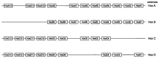
Another example of intriguing patterns of gene arrangement is the hox gene family in man and the mouse, shown in Figure 15.12. The genes in this family code for factors that determine the segmental pattern of organization of the developing embryo. The family is
Figure 15.12 Organization of homeobox (hox) genes in the mammalian genomes. All genes in all four clusters are transcribed from left to right.
548 RESULTS AND IMPLICATIONS OF LARGE-SCALE DNA SEQUENCING
complex, and dispersed on a number of different chromosomes. Two aspects of the organization of the family are striking. First, it is so well conserved between the two species. Second, the spatial order of the genes within the family is the same as the order of the segments in the embryo that these genes affect. It is as if, for some totally unexplained reason, the map of the structure of the gene family is an image of the map of the function
of that family.
A final example of functionally interesting gene arrangements is seen in a number of the members of the immunoglobulin superfamily including the light and heavy chains of antibodies, and several chains of the T-cell receptor. Here large numbers of related genes
are grouped together, mostly in a single continuous segment of |
a chromosome. The rea- |
|
son for this is probably to assist the rearrangement of these |
genes, which takes place by |
|
DNA splicing to form mature expressed genes for antigen-specific proteins. If other re- |
||
gions of the genome are found with very large clusters of similar genes, one may well |
||
suspect |
that somatic DNA rearrangement or some other unusual |
biological mechanism |
will be at play with these genes. |
|
|
A |
totally different view of global function afforded by |
complete physical maps and |
DNA sequences is the ability to compare these physical structures of DNA with the ge- |
||
netic map. An example is shown in Figure 15.13 for yeast chromosome III. There are |
||
clearly |
some regions where meiotic recombination is much more |
frequent than average |
and others where it is greatly suppressed. We do not yet understand the origin of these ef- |
||
fects. One possibility is just the presence or absence of local DNA sequences that constitute recombination hot spots. However, there are other more global possibilities.
Recombination may correlate with overall transcriptional |
activity, since highly tran- |
scribed chromatin is more open and accessible to all types of enzymes including those re- |
|
sponsible for recombination. Thus there may be positional relationships between gene |
|
function and recombination, and thus gene evolution, that |
we still know nothing about |
today. |
|
SEARCHING FOR THE BIOLOGICAL FUNCTION OF GENES
Most biologists, when they think of biological function in the context of the genome project, are referring to the function of individual genes. A common criticism of the genome project is that it is relatively useless to know the DNA sequences of genes without strong prior hints about their function. Most traditional molecular genetics begins with a function of interest and attempts to find the genes that determine or affect that function. This traditional view of biology is contrasted with the challenge posed by genome research in
Figure 14.1, |
which can well serve as a paradigm for all of biology. In genome research |
|||
we will discover DNA sequences with no a priori known function. Our current ability to |
|
|||
translate these |
DNA sequences correctly into protein sequences |
is excellent, |
as |
we |
showed earlier, by using GRAIL or other powerful algorithms. Our current ability to take |
||||
these protein sequences and draw immediate inferences about their |
possible function |
is |
|
|
well illustrated |
by the example in Figure 15.14 |
a . Except |
for those rare readers of this |
|
book who are conversant in Dutch, this passage is largely unreadable. However, the frustrating aspect is that the passage is not totally unreadable. Because a number of scientific terms are cognates in Dutch and English, certain features stand out—one knows the passage has something to do with protein structure, but the full impact of the message is completely lost.

SEARCHING FOR THE BIOLOGICAL FUNCTION OF GENES |
549 |
Figure 15.13 |
A comparison of the genetic and physical map of the yeast |
S. cerevisiae. |
Ingewikkelde en grote biologische macro-moleculen kunnen spontaan
in hun meest stabiele conformatie vouwen. Helaas, ontbreekt ons de kennis om dit proces te voorspellen want de gevouwen strutuur kan belangrijke aanwijzingen
over die functie van het molecuul bevatten.
(a)
We know that large biological molecular can fold into their most stable state spontaneously but we really have little ability at present to predict this folding. Our ignorance is most unfortunate since the folded structure may contain important clues on how the molecule functions.
|
|
(b) |
|
Figure 15.14 |
An analogy for the current |
(a) and desired future |
(b) ability to interpret DNA se- |
quence in terms of its likely biological function. |
|
|
|
550 |
RESULTS AND IMPLICATIONS OF LARGE-SCALE DNA SEQUENCING |
||
|
When the passage in Figure 15.14 |
a is translated into English, it provides an important |
|
clue to one direction that can help find functional clues (Fig. 15.14 |
b ). Considerable expe- |
||
rience to date shows that protein three-dimensional structures are better conserved during |
|||
evolution than protein sequences. A great deal of |
current research effort is being devoted |
||
to improving our ability to infer possible protein structures from the sequences of sets of |
|||
related proteins, provided that at least one of them has a known three-dimensional struc- |
|||
ture. As our ability to do this improves, and as the number of different classes of protein |
|||
structures has one or more members successfully studied at high-resolution by X-ray |
|||
crystallographic or nuclear magnetic resonance |
techniques, the prospects |
of stepping |
|
quickly from a sequence to a realistic, if not exact, model of the structure should improve markedly. However, just knowing a three-dimensional structure does not immediately provide definitive clues to function. It simply makes comparisons between a protein of
unknown function and the set of |
proteins of known function more powerful and more |
|
likely to yield useful insights. |
|
|
Today, when a new segment of DNA sequence is determined, the first thing that is al- |
||
most always done with it is to compare it to all |
other known DNA sequences. The pur- |
|
pose is to see if it is related to anything already known. By related, we mean, that there is |
||
a statistically significant similarity to one or more preexisting DNA sequences. The defin- |
||
ition of what statistically significant means in the context of sequence comparisons is not |
||
universally accepted despite decades of work in this area. Obviously, at one extreme, one |
||
may find that a new sequence is virtually identical to a preexisting one. Unless the two se- |
||
quences derive from very similar but not identical organisms, the finding of near identity |
||
means true identity with the differences due to sequencing errors, or a new member of a |
||
gene family, or an example of proteins very strongly conserved in evolution, like the his- |
||
tones. At the other extreme, a new sequence may match nothing to within whatever local |
||
standards of minimal homology are considered operative. |
||
Most often, however, when |
a new DNA sequence is compared with the current data |
|
base of more than 1000 Mb of DNA, some slight or significant sequence homology is |
||
found. For coding sequences, it is usually much more powerful to search after translation |
||
of DNA to protein. This translation loses very little functional information; it gains con- |
||
siderable statistical power because the noise caused by the degeneracy of the genetic code |
||
is blanked out. Thus consider, for example, two arginine codons like AGG and CGA in a |
||
corresponding place on two sequences; the only evidence for similarity is the G in posi- |
||
tion 2, which has roughly one chance in four of |
occurring randomly. In contrast, posing |
|
an arginine opposite an arginine at the same place in a protein sequence has, very crudely, |
||
only one chance in 20 of occurring randomly. (In reality the statistical differences are not |
||
this great because amino acids with six possible codons, like arginine, also tend to occur |
||
much more often than average.) |
|
|
A statistically significant match between a |
new sequence and some preexisting se- |
|
quence implies some or all of the following possibilities: similar function, similar struc- |
||
ture, or evolutionary relatedness. It is not easy to sort out these different effects. However, |
||
one encouraging feature of such global sequence searches is that their effectiveness ap- |
||
pears to be increasing markedly and rapidly as the database grows. Ten years ago Russell |
||
Doolittle noted that a new protein sequence had |
a 25% chance of matching something |
|
else in the databases. Currently the odds are considerably better than this. From the first |
||
bacterial sequencing projects described earlier in this chapter, between 54% and 78% of |
||
the ORFs found showed hints of homology in structure or function with something else in |
||
the data base. With the |
S. cerevisiae |
ORFs on chromosome III, 42% gave hints of homol- |

|
|
|
|
|
|
|
|
|
|
METHODS FOR COMPARING SEQUENCES |
551 |
ogous structure or function of which 14% were deemed really quite strong. In the case of |
|
||||||||||
C. elegans, |
|
where |
more |
extensive data are available, 45% of the ORFs were reported to |
|
||||||
be relatable to existing databases. It seems likely that in a few years it will be the odd new |
|
||||||||||
sequence that does not immediately match something known. While it is too early to be |
|
||||||||||
sure how rapidly this goal will be achieved, there is room for considerable optimism at |
|
||||||||||
present. |
|
|
|
|
|
|
|
|
|
|
|
METHODS |
FOR COMPARING SEQUENCES |
|
|
|
|||||||
Entire books have been written about the relative merits of different approaches to align- |
|
||||||||||
ing sequences and testing their relatedness (Waterman, 1995; Gribokow and Deveraux, |
|
||||||||||
1991). The topic is actually quite complex because the nonrandom nature of natural DNA |
|
||||||||||
sequences greatly confounds attempts to construct simple statistical tests of relatedness. |
|
||||||||||
Here our goal will be to present |
the basic notions of how sequences are compared and |
|
|||||||||
what these comparisons mean. Sequences are strings of symbols. Any two strings can be |
|
||||||||||
compared |
by |
direct |
alignment |
and |
the |
use of |
scoring |
criteria for similarity. For two |
|
||
strings of length |
|
|
n |
and |
m |
there |
are |
2(n m 1)possible continuous alignments, by |
|
||
which we mean that no gaps are allowed in either string. Of course many of these align- |
|
||||||||||
ments are fairly trivial and |
uninteresting because the strings will barely overlap. The |
|
|||||||||
moment gaps are allowed on one or both strings, the number of alignments rises in a |
|
||||||||||
combinatorial manner to reach heights that can test the power of the fastest existing su- |
|
||||||||||
percomputers if the problem is not handled intelligently. |
|
|
|||||||||
An example of a very simple |
case in which two very similar DNA sequences are |
|
|||||||||
aligned is shown in Figure 15.15. In this case the alignment needed to maximize the ap- |
|
||||||||||
parent similarity between the two sequences is obvious. What is less obvious is the sort of |
|
||||||||||
score to give such an alignment. The simplest scoring scheme is black and white: Grade |
|
||||||||||
all identities the same and all differences the same. However, this makes little sense from |
|
||||||||||
either a biological or a statistical vantage point. As far as biology is concerned, if, for ex- |
|
||||||||||
ample, we are looking at the functional relatedness of proteins coded for by these se- |
|
||||||||||
quences, or if we are looking at possible evolutionary relationships between them, trans- |
|
||||||||||
versions |
(interchange |
of |
a purine and a pyrimidine) should be weighted as more |
|
|||||||
consequential differences than transitions (interchange between two pyrimidines or two |
|
||||||||||
purines). This is because the rate of transversion mutations is much less than the rate of |
|
||||||||||
transitions, |
and |
the |
genetic |
code appears to have evolved so that effects of transversions |
|
||||||
on the resulting amino acids |
are more functionally disruptive than the effect of transi- |
|
|||||||||
tions. For example, many synonymous codons are related by a transition in their third po- |
|
||||||||||
sition. But the example goes much deeper; for example, codons for different hydrophobic |
|
||||||||||
amino acids are also related mostly by transitions. |
|
|
|
||||||||
Figure 15.15 A simple example of a comparison between two putatively related nucleic acid se-
quences and two ways in which their relatedness could be scored, |
S transition and |
V trans- |
version. |
|
|

552 RESULTS AND IMPLICATIONS OF LARGE-SCALE DNA SEQUENCING
To take statistical factors into account in estimating the significance of a mismatch or a match purely at the DNA level, we have to consider the relative frequency of each residue
in the strings being compared. For example, sequences rich in A’s will show large numbers of A’s matched with A’s, just by chance. In order to take this into account, and to add issues like transitions and transversions, one needs to employ a scoring matrix. This is il-
lustrated in Figure 15.16 |
a . The 4 |
4 scoring matrix for nucleic acid comparisons allows |
||||||
for any possible weight to be assigned to a particular set of bases at |
an |
alignment posi- |
||||||
tion. Generally, the same scoring matrix is used for every alignment position, although |
||||||||
there is no reason why one should have to do this, nor is there any reason why it is desir- |
||||||||
able except for simplicity. Think ahead to the alignment of protein |
sequences |
where |
||||||
residues on exterior loops can be quite variable without perturbing the overall structure. |
||||||||
Therefore, if one had some way of knowing a priori that a residue was |
in a loop as op- |
|||||||
posed to a helix or sheet, one could adjust the weighting factors accordingly. This exam- |
||||||||
ple illustrates the complex interplay between sequence and structure information that re- |
||||||||
ally has to occur in very robust comparison algorithms. |
|
|
|
|
||||
The simplest possible DNA scoring matrix, corresponding to the rule used in Figure |
||||||||
15.15 is just a set of identities with no correction for overall base composition (Fig. |
||||||||
15.16b ). The general case would consist of a set of elements |
|
|
|
a ij that are all different, ex- |
||||
cept that the matrix should be symmetrical; each |
|
|
a ij a ji since we have no way, in com- |
|||||
paring just two proteins, to favor one sequence over another. The elements |
|
|
a ij must incor- |
|||||
porate all of our biological and statistical prejudices. When |
protein |
sequences are |
||||||
compared, |
the scoring matrices |
can become more complicated. First of |
all, |
the |
matrix |
|||
must be 20 |
20 instead of 4 |
4. It can be as simple as an identity matrix, just as in the |
||||||
case for nucleic acids, but a much more accurate picture will incorporate statistical infor- |
||||||||
mation about the relative frequency of amino acids. This immediately raises one serious |
||||||||
problem: Does one use the amino acid composition of the two proteins in question to |
||||||||
construct the scoring matrix, or does one use the amino acid compositions of all known |
||||||||
proteins, or all known proteins |
from the particular species involved? |
One can |
elaborate |
|||||
the problem even further by asking whether the nonrandomness of dipeptide frequencies |
||||||||
should be considered in making statistical evaluations for the scoring matrix. There are no |
||||||||
simple answers to these questions. |
|
|
|
|
|
|
|
|
Most commonly, with protein sequence comparisons, one incorporates |
information |
|||||||
about amino acid physical properties into the values of the elements of the scoring matrix. |
||||||||
Thus, for example, interchanges among ile, leu, and val, or ser and thr, among proteins |
||||||||
known to be related in structure |
and function |
are |
very commonly seen and are presum- |
|||||
ably mostly innocuous. Examples of two real scoring matrices are shown in Figure 15.17.
Figure 15.16 |
Comparison matrices between two nucleic acid sequences. |
(a) A general matrix. |
(b) |
The simplest possible matrix.

METHODS FOR COMPARING SEQUENCES |
553 |
Figure 15.17 |
An example of actual scoring matrices for protein sequences that takes into account |
||
the similar properties of certain |
types of amino acids. |
(a) the Blosum G2 matrix used by BLAST |
|
(Henikoff and Henikoff, 1993). |
(b) The structural (STTR) matrix of Shpaer et al. (1996). |
||

554 RESULTS AND IMPLICATIONS OF LARGE-SCALE DNA SEQUENCING
The values of these elements obviously vary over a wide range. However, despite their different origins, the two matrices are fairly similar.
There is still one additional complication that must be dealt with. This is especially serious when one wishes to estimate the evolutionary relatedness of two proteins or DNAs.
Here a yardstick that is often used as a time scale for evolutionary divergence is the probable average number of mutations needed to convert one sequence into the other. Such comparisons among very similar proteins or nucleic acids are relatively simple. Differences seen are presumably real, and similarities are also presumed real. However, when more distant sequences are compared, an apparent similarity has an increasing
chance of just being |
a statistical event, or a reversion. For example, as shown in Figure |
15.18 two matching A’s could be a true identity (no mutations) or a reversion (a minimum |
|
of two mutations). The |
more distantly related the two sequences, the more the latter pos- |
sibility has to be weighted. Ways of doing |
this for simple identity comparison matrices |
were developed several decades ago by Jukes |
and Cantor, and later elaborated consider- |
ably to take into account statistical effects and similarities in residue properties. The kind of matrix needed in a very simple case is shown in Figure 15.19. It adjusts the relative weights of comparisons as a function of the average extent of differences between the two sequences. The problem of choosing an ideal comparison matrix, which deals with all of
these interrelated issues, is still not a simple one.
Once a comparison matrix is chosen, it can be used to evaluate the relative similarity seen in all possible alignments between two strings. When gaps (caused by a putative insertion or deletion, or a pure statistical artifact) are allowed, the problem of actually enumerating and testing all possible comparisons becomes computationally extremely de-
Figure 15.18 Difficulties in sequence comparisons when the goal is to estimate the probable number of mutations that have occurred to derive one sequence from another (or both from a com-
mon ancestor).
Figure 15.19 |
A simple scoring matrix that takes into account the average differences between two |
|
|
||
sequences and allows for the possibility of revertants. Where |
a |
1/4(1 e 4d/3). The parameter |
d |
||
is a measure of the true evolutionary distance between two sequences being compared. It is the av- |
|
|
|
||
erage number of mutations per site that separate one sequence from the other. In the limit |
|
the |
d |
: 0 |
|
matrix becomes equal to |
the right-hand panel of Figure 15-16. In the limit |
all |
of the ele- |
d : |
|
ments of the matrix become equal to 1/4. This means that the sequences have diverged so much that one is essentially comparing two random strings.

|
|
|
|
|
|
METHODS FOR COMPARING SEQUENCES |
555 |
|||
manding. Figure 15.20 shows a very simple example. The issue is how to test the likeli- |
|
|
||||||||
hood that the postulated gap results in a statistically significant improvement in the align- |
|
|||||||||
ment score of the two sequences. Obviously there must be a statistical penalty attached to |
|
|
|
|||||||
the use of such a gap, since it greatly increases the number of possible comparisons, and |
|
|||||||||
thus the chance of finding, at random, a comparison with a score better than some arbi- |
|
|||||||||
trary value. |
|
|
|
|
|
|
|
|
|
|
From a practical point of view, it is impossible to test all possible gap numbers and lo- |
|
|||||||||
cations. One way to deal with this problem is to compare two sequences through smaller |
|
|
|
|||||||
windows, sets of successive residues, rather than |
globally (Fig. 15.21). With two |
strings |
|
|||||||
of length |
n |
and |
m |
, and a window of length |
|
L, there are |
(n |
L 1)(m L 1)possible |
|
|
comparisons to be done. This is not a major task for strings the sizes of typical genes. For |
|
|||||||||
each choice of window, two substrings of length |
|
L are compared, without gaps. The score |
|
|||||||
for this comparison is calculated as the sum over the |
matrix |
elements |
|
|
a ij for each of the |
L |
||||
residues pairs. To provide a visual overview of the comparison, it is usually convenient to |
|
|
|
|||||||
plot all scores above some threshold value as a dot in a rectangular field formed by writ- |
|
|
||||||||
ing one sequence along the horizontal axis and the other along the vertical axis. Any point |
|
|
|
|||||||
in the field corresponds to an alignment of |
|
L residues positioned at particular residue po- |
|
|||||||
sitions in the two sequences. This kind of dot matrix |
plot is shown, schematically |
|
in |
|
||||||
Figure 15.22, and a real example of a sequence |
comparison at the DNA level for two |
|
|
|||||||
closely related |
viruses, |
SV40 and polyoma is |
given |
in Figure 15.23. Any |
regions |
with |
|
|||
Figure 15.20 A simple case of two sequences potentially related by an insertion or a deletion.
Figure 15.21 Window selection on a single sequence assists in comparisons.
Figure 15.22 An example of the comparison of two proteins or DNAs using windows on each, evaluated with a scoring matrix. Shown as dots are all comparisons that score above a selected threshold.