

|
|
|
|
|
|
|
DIAGNOSTICS AT |
THE DNA |
LEVEL |
453 |
|
TABLE 13.3 Forty-Three Somatic Mutations of Colorectal Tumors in the APC Gene |
|
|
|
|
|||||||
|
|
|
|
|
|
|
|
||||
C113(F) |
142 |
a |
a tag/CTG |
: atag/CTG |
|
|
Splice acceptor |
||||
C31, C124(F) |
213 |
CGA |
|
: T |
GA |
|
|
|
Arg |
: Stop |
|
C24 |
279 |
aatttttag/GGT |
|
|
: agtttttag/GGT |
|
Splice acceptor |
||||
C47 |
298 |
C |
ACTC |
: CTC |
|
|
AC deletion |
||||
C108(F) |
302 |
CGA |
|
: T |
GA |
|
|
|
Arg |
: Stop |
|
C135 |
438 |
CAA/gtaa |
|
|
: CAA/g |
c aa |
|
Splice donor |
|||
C33 |
516 |
|
AAG/gt |
|
: AAG/ tt |
|
|
Splice donor |
|||
C28 |
534 |
AAA |
|
: T |
AA |
|
|
|
Lys |
: Stop |
|
C10 |
540 |
TTA |
: TT |
AT |
|
|
A insertion |
||||
C37 |
906 |
T |
C TG |
|
: TTG |
|
|
|
C deletion |
|
|
A128(F) |
911 |
GAA |
|
: G |
G |
A |
|
|
Glu |
: Gly |
|
C23 |
1068 |
TCAAGGA |
|
: GGA |
|
|
TCAA deletion |
||||
C11, C15 |
1114 |
CGA |
|
: T |
GA |
|
|
|
Arg |
: Stop |
|
C20 |
1286 |
GAA |
: T |
AA |
|
|
|
Glu |
: Stop |
||
A53 |
1287 |
ATA |
: A |
ATA |
|
|
|
A insertion |
|||
C27 |
1293 |
ACACAGGAAGCAGATTCT |
|
31 bp deletion |
|||||||
|
|
GCTAATACCCTGC |
AAA |
: AAA |
|
|
|||||
C7, C21 |
1309 |
G |
AAAAGAT |
: GAT |
|
|
AAAGA deletion |
||||
C14 |
1309 |
GAA |
|
: T |
AA |
|
|
|
Glu |
: Stop |
|
A41 |
1313 |
ACT |
: G |
CT |
|
|
|
Thr |
: Ala |
||
C31, C42 |
1315 |
TCA |
|
: T A |
|
|
|
Ser |
: Stop |
||
A44 |
1338 |
CAG |
|
: T |
AG |
|
|
|
Gln |
: Stop |
|
C22 |
1353 |
GAATTTTCTTC |
: TTC |
|
8 bp deletion |
||||||
A56 |
1356 |
|
TCA |
: T G A |
|
|
|
Ser |
: Stop |
||
C4, C27 |
1367 |
CAG |
|
: T |
AG |
|
|
|
Gln |
: Stop |
|
C10 |
1398 |
AG TCG |
|
: TCG |
|
|
AG deletion |
|
|||
C19 |
1398 |
AG |
T C |
|
: AGC |
|
|
|
T deletion |
|
|
A43 |
1411 |
A |
G TG |
|
: ATG |
|
|
|
G deletion |
|
|
C16 |
1420 |
CC |
C A |
|
: CCA |
|
|
|
C deletion |
|
|
C40, A52(F) |
1429 |
GAA |
|
: T |
AA |
|
|
|
Gln |
: Stop |
|
C29 |
1439 |
C |
C TC |
|
: CTC |
|
|
|
C deletion |
|
|
C37 |
1446 |
G |
CTCAAACCAAGC |
: GGC |
10 bp deletion |
||||||
A50(F) |
1448 |
T |
T AT |
|
: TAT |
|
|
|
T deletion |
|
|
A49(F) |
1465 |
AG TGG |
|
: TGG |
|
|
AG deletion |
|
|||
C23 |
1490 |
C |
ATT |
|
: CTT |
|
|
|
A deletion |
|
|
C12 |
1492 |
GC |
C A |
: GCA |
|
|
|
C deletion |
|
||
A41 |
1493 |
ACAGAAAGTAC TCC |
: TCC |
11 bp deletion |
|||||||
C3 |
1513 |
GAG |
: T |
GAG |
|
|
|
T insertion |
|
||
|
|
|
|
|
|
|
|
|
|
|
|
Source: Adapted from Miyoshi et al. (1992).
If we had the ability to do very large-scale DNA sequencing, genetic diseases could be diagnosed by this technique with great power but still not without difficulties. We would still have to develop effective ways to distinguish, for newly found alleles, whether they were just harmless polymorphisms or true disease-causing alleles. While some guidelines for how this might be done were presented earlier in the chapter, it will be hard to do this in general without considerable information about the function of the protein product of the gene. An example of the complex spectrum of spontaneous mutations seen in the hu-
man factor IX gene responsible for hemophilia B is shown in Table 13.4. These results
454 |
FINDING GENES |
AND MUTATIONS |
|
|
|
|
|
||
|
TABLE |
13.4 Summary of Sequence Change in 260 Consecutive Cases of Hemophilia B |
|
|
|||||
|
|
|
|
|
|
|
|
|
|
|
|
|
|
|
|
|
|
Number |
Percentage |
|
|
|
|
|
|
||||
|
1. Number with sequence changes in the eight regions of likely |
249 |
|
96 |
|
||||
|
functional significance |
|
|
|
|
|
|
||
|
2. Of those with sequence changes, number of independent |
182 |
|
73 |
|
||||
|
mutations |
a |
|
|
|
|
|
|
|
|
|
|
|
|
|
|
|
||
|
3. Of independent mutations, number with a second sequence |
6 |
|
3 |
|
||||
|
change |
|
|
|
|
|
|
|
|
|
4. Type of independent mutation: |
|
|
|
|
|
|||
|
Transitions at CpG |
|
|
|
|
48 |
26 |
||
|
Transitions at non-CpG |
|
|
|
|
65 |
36 |
||
|
Transversions at CpG |
|
|
|
|
8 |
4 |
||
|
Transversions at non-CpG |
|
|
|
35 |
19 |
|||
|
Small deletions and insertions ( |
50 bp) |
|
|
15 |
8 |
|||
|
Large deletions ( |
50 bp) |
|
|
|
10 |
6 |
||
|
Large insertions |
|
|
|
|
1 |
0.6 |
||
|
5. Location of independent mutations: |
b |
|
|
|
|
|||
|
|
|
|
|
|
||||
|
Promoter |
|
|
|
|
|
1 |
0.5 |
|
|
Coding sequence |
|
c |
|
|
|
163 |
86 |
|
|
|
|
|
|
|
||||
|
Splice junctions |
|
|
|
|
12 |
6 |
||
|
Intron sequences away from splice junctions |
|
|
1 |
0.5 |
|
|||
|
Poly A region |
|
|
|
|
|
0 |
— |
|
|
Unlocalized (total gene deletions) |
|
|
|
5 |
3 |
|||
|
Unknown |
b |
|
|
|
|
8 |
4 |
|
|
|
|
|
|
|
||||
|
6. Functional consequences of observed independent mutations |
|
|
|
|
||||
|
Protein with amino acid substitutions |
|
|
114 |
63 |
||||
|
Garbled protein (truncated, frameshifted or partial or full |
54 |
|
30 |
|
||||
|
|
deletion of amino acids) |
|
|
|
|
|
||
|
Abnormal splicing |
|
|
|
|
13 |
7 |
||
|
Decrease expression |
|
|
|
|
1 |
0.6 |
||
|
|
|
|
|
|
|
|
||
|
Source: |
Adapted from Sommer et al. (1992). |
|
|
|
|
|
||
|
a Recurrent mutations were judged independent if the |
haplotypes differed. In a |
few cases recurrent |
mutations |
|
|
|||
|
with the same haplotype were judged independent because the origin of mutation was determined. In four pa- |
|
|
||||||
|
tients recurrent mutations were judged independent because the races of the individuals were different. |
|
|
|
|||||
bAssumes that 11 patients with unknown mutations have the same frequency of independent mutations as patients in which the mutation could be defined (73%). Thus eight independent mutations should be unknown.
cIncludes partial gene deletions that affect the coding region.
clearly indicate that no single test at the DNA level, even complete DNA sequencing, would be capable of 100% certain diagnoses. It is difficult to measure heterozygous positions with typical gel-based sequencing, and haplotypes of compound heterozygotes can-
not be determined at all.
The difficulty of DNA analysis of cancers includes all of these problems, but it is confounded by the heterogeneity of typical tumor tissue. For very early onset diagnosis of somatic cancer, one would need to distinguish, potentially, any altered nucleotide, in a complex gene, present in only a minute fraction of the cells in a sample. It is not easy to see how this could be accomplished by directly DNA sequencing alone. In all these cases, the
task is much simpler if only a finite number of specific sequence alleles are correlated with the disease. Then one can set up specific assays for the alleles, and some such assays

|
|
|
|
|
|
ANALYSIS OF DNA SEQUENCE DIFFERENCES |
455 |
||
seem capable of dealing with the sorts of heterogeneous samples encountered in tumors. |
|
|
|||||||
The emergence of specific cancer or disease-associated alleles can also be tested for in |
|
||||||||
easily assayable fluids. For instance, the fingerprint of prostate tumor cells has been de- |
|
||||||||
tected in urine, and those of head and neck tumors have been detected in saliva and blood. |
|
|
|||||||
ANALYSIS |
OF |
DNA |
SEQUENCE |
DIFFERENCES |
|
|
|
|
|
The examples described in the previous section clearly indicate the need to be able to an- |
|
||||||||
alyze a stretch of DNA |
sequence to look for abnormalities that might be as small as |
sin- |
|
||||||
gle base pair. If the DNA target is just a few thousand base pairs, this search can be |
done |
|
|||||||
by direct sequencing. If the target is much larger, direct sequencing with current methods |
|
||||||||
is impractical. In this section we explore the present status of methods that can |
detect |
|
|||||||
changes in DNA as small as single base pairs, with less effort than would be required for |
|
||||||||
total DNA sequencing. Many of these methods resort to the formation of DNA heterodu- |
|
|
|
||||||
plexes to facilitate the screening for differences between a test sequence and a standard. |
|
||||||||
Figure |
13.14 |
a |
shows, schematically the three possible genotypes that must |
be distin- |
|
||||
guished in making a genetic diagnosis. In general, an individual tested could be normal |
|
||||||||
(dd), heterozygous for the disease allele (dD), or homozygous for the disease allele (DD). |
|
||||||||
If the disease is dominant, one usually expects the affected to be a heterozygote. If one is |
|
||||||||
testing for a carrier status, the test is really looking to see if the individual in question is a |
|
||||||||
heterozygote. In |
either |
of |
these cases, a |
normal DNA duplex is present that can serve |
as |
|
|||
an internal control for the possible presence of an altered duplex. DNA from the region of |
|
|
|||||||
interest |
can |
be |
prepared |
directly from |
genomic material by PCR, assuming |
enough |
|
||
known sequence exists to design suitable primers. If this DNA is melted and the separated |
|
|
|||||||
strands are allowed to reanneal, four distinct products will be formed (Fig. 13.14 |
|
b ). Two |
|||||||
of these are the perfectly paired normal and abnormal duplexes. The remaining two are |
|
|
|||||||
heteroduplexes composed of one normal and one abnormal strand. Any DNA sequence |
|
|
|
||||||
differences between these species will lead to imperfections in the duplex because one or |
|
||||||||
more base pairs will be mismatched. |
|
|
|
|
|||||
Figure 13.14 |
Detection of a disease allele as a heteroduplex. ( |
a ) Three genotypes that must be dis- |
|||
tinguished |
in disease |
diagnosis. ( |
b ) Heteroduplex formation by melting and |
reannealing |
DNA from |
a recessive |
carrier or |
a dominant heterozygote. ( |
c ) Heteroduplex |
formation by |
mixing DNA from a |
homozygous recessive with DNA from a normal individual.
456 FINDING GENES AND MUTATIONS
If the disease in question is recessive, the usual question asked is whether the particular individual being tested is homozygous for the disease allele or heterozygous. Thus a
minimal test would be to proceed |
exactly as described above, except that now, presence |
||||||
of |
heteroduplex |
indicates |
that |
the |
individual |
is a carrier, unaffected for the disease. |
|
However, this |
test would |
be ambiguous because |
absence of heteroduplex would imply |
||||
that |
either the |
individual |
in question is a homozygous normal or a homozygous affected. |
||||
An additional test is required to resolve this |
ambiguity. This second test is designed as |
||||||
shown in Figure |
13.14 |
|
c . DNA from |
the individual to be tested is mixed with a standard |
|||
DNA sample from a person previously shown to be normal, not a carrier. If the test indi- |
|||||||
vidual carries the disease, four DNA products will be formed; two of these will be het- |
|||||||
eroduplexes. If |
|
the test individual is |
normal, no heteroduplex products will be produced. |
||||
Thus the tests shown in Figure 13.14 reduce the problem of detecting DNA sequence alterations to the problem of detecting heteroduplex DNA.
We will shortly describe a wide variety of techniques that have varying success in distinguishing between DNA heteroduplexes and homoduplexes. One caveat in using these
methods for genetic testing must be noted. Successful heteroduplex detection will find |
|||
any DNA alterations, whether or not these are disease alleles or |
harmless polymorphisms. |
||
Thus |
what |
heteroduplex detection does is indicate the presence |
of a DNA sequence vari- |
ant. |
Once |
this is found, DNA sequencing will frequently be needed to examine the char- |
|
acteristics of the particular variant discovered. Thus the strategy used is to apply a very simple test that can scan large DNA regions to see if any sequence variations exist. If none are found, and the test is reliable, one need go no further. If differences are discovered, then usually a more robust test will need to be applied, but the screening will have narrowed down the DNA target to a much smaller region. For example, PCR can be used
to examine the exons of a complex gene one at a time. If a sequence variation is discovered in a single exon, at worst one would have to sequence the DNA of that exon to complete the diagnosis.
HETERODUPLEX DETECTION
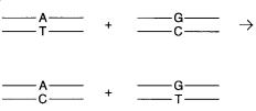
The difficulty in designing schemes to detect heteroduplexes is that many possibilities can arise, even from a single altered base pair. This is shown in Figure 13.15. Any mixture of two DNAs with a single base pair difference produces two different heteroduplexes with a
single base mismatch. In all, there are eight possible single base mismatches: A–C, A–A, A–G, C–C, C–T, T–T, T–G, G–G, and an acceptable test would have to be able to detect them all. The ideal test would not only detect them, but it would also reveal which exact mismatches were present. A potential complication is that each heteroduplex occurs
Figure 13.15 |
A single site mutation will serve to generate the formation of two different |
heteroduplexes. |
|
HETERODUPLEX DETECTION |
457 |
within the context of a specific DNA sequence, and the identity of the neighboring base pairs could easily modulate the properties of the heteroduplex. Not much is known about this at present.
In practice, the formation of heteroduplexes from a diploid sample will produce a pair of mismatches. For single base pair differences there are only four possibilities, and each
gives a different and discrete set of heteroduplexes. Thus a |
test that detected a specific |
half of the possible heteroduplexes would suffice: |
|
M UTATION |
H ETERODUPLEXES |
A–T to T–A |
A–A and T–T |
G–C to C–G |
G–G and C–C |
A–T to G–C |
G–T and A–C |
A–T to C–G |
A–G and C–T |
Thus, for example, a method that could identify a mispaired T or G but not A or C would suffice to spot the presence of a heteroduplex, but it would probably not have enough resolving power to identify the exact heteroduplex present.
The single-base, mismatched heteroduplexes just illustrated are actually the most difficult case to detect by the methods currently available. Larger mismatches or heteroduplexes arising from insertions or deletions lead to much larger perturbations in the DNA double helical structure, and these are easier to reveal by physical and chemical or enzymatic methods. The principle complication is that the number of possible heteroduplexes
becomes rather larger. There are four possible single base |
|
insertions |
or deletions, but |
||
these are likely to be susceptible to complexities caused by |
the local |
sequence |
context. |
||
For example, in the sequence shown below, two altered mismatched structures compete |
|||||
with each other. |
|
|
|
|
|
A–T |
A–T |
|
|
A–T |
A–T |
G–C |
C |
|
G–C |
||
G–C |
9: G–C |
|
;: G–C |
C ;9 G–C |
|
T–A |
T–A |
|
|
T–A |
T–A |
|
|
|
|
||
The genetic consequences of the two different structures shown above are identical; however, the presence of two alternate heteroduplex structures could complicate the analysis.
Much |
more work needs to be done to |
characterize the properties of such structures in |
|
more |
detail. This will have to be |
done before the overall accuracy of any |
proposed |
method of heteroduplex detection can be validated for clinical use. |
|
||
|
At least six different basic methods for detecting heteroduplex DNA have been de- |
||
scribed. All of these tests work well |
in some cases. However, none have yet been |
proved |
|
to be generally applicable to all possible heteroduplexes. A key issue in these tests is how
large |
a |
DNA target can be examined directly. The larger the target, the fewer fragments |
|||||
will |
be |
needed to cover |
a |
whole gene. However, if targets are too large, |
they |
may |
have |
such |
a |
high probability |
of |
containing a phenotypically silent polymorphism |
that |
the |
ad- |
vantage of the test as a primary screen will be lost, since many fragments will test posi-
tive. The first four tests, illustrated in Figure 13.16, all have potentially similar characteristics, and all will work, in principle, on very large DNA targets. A straightforward and
direct approach is to use single-strand-specific DNases like S1 nuclease to cleave at the
458 FINDING GENES AND MUTATIONS
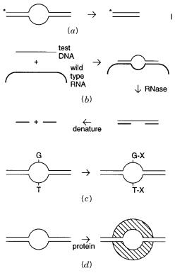
Figure |
13.16 |
Four different methods |
for |
direct detection of heteroduplex DNA. ( |
|
a ) |
Nicking with |
||||
S1 nuclease. ( |
b ) Trimming and nicking an RNA-DNA hybrid with ribonuclease. ( |
|
c ) Reaction of un- |
||||||||
paired |
bases |
with |
organic |
molecules |
like carbodiimides. ( |
d ) Binding |
of |
mut S protein to |
the site of |
||
the mismatch. |
|
|
|
|
|
|
|
|
|
||
mismatched |
bases |
in a heteroduplex (Fig. 13.16 |
a ). Then the |
resulting |
shortened DNA |
|
|||||
fragment could be detected by a Southern blot or by PCR. The difficulty with this ap- |
|
|
|||||||||
proach is that no known combination of enzyme and reaction conditions allows reliable |
|
|
|
||||||||
cleavage at single base mismatches. Larger mispaired targets are needed before cleavage |
|
|
|
||||||||
becomes efficient and selective. Other nucleases that look very promising for such studies |
|
|
|
||||||||
include bacteriophage T4 endonuclease VII. |
|
|
|
|
|
|
|||||
RNase nicking can be used as an alternative to DNase nicking. Here a single strand of |
|
|
|
||||||||
the DNA to be tested is annealed with RNA made from a DNA sample representing the |
|
|
|
||||||||
normal allele (Fig. 13.16 |
b ). This is easily accomplished, for example, by subcloning that |
|
|||||||||
allele downstream from a strong in vitro promoter like that for T7 RNA polymerase. One |
|
|
|
||||||||
can produce either internally labeled RNA, |
and |
look for |
two shorter fragments as a sign |
|
|
|
|||||
of fragmentation, |
or end-labeled RNA, and look for one |
shorter fragment. In this latter |
|
|
|
||||||
case it is necessary to have the test DNA extend beyond the labeled end of the RNA; oth- |
|
|
|
||||||||
erwise, the RNase will remove the label. Some workers swear by the reliability and sensi- |
|
|
|
||||||||
tivity of the RNase approach, but many others have apparently been unable to use it suc- |
|
|
|
||||||||
cessfully. |
|
|
|
|
|
|
|
|
|
|
|
Chemical methods can be used instead of enzymes to mark or to cleave at the site of a |
|
|
|
||||||||
mismatch. A particularly effective approach has been the use of water-soluble carbodi- |
|
|
|
||||||||
imides |
which can |
react |
with mismatched T |
or |
G (Fig. |
13.16 |
c ). These compounds |
are |
|||
|
|
|
|
|
|
HETERODUPLEX |
DETECTION |
|
459 |
|
available radiolabeled, so one can detect the presence of a mismatch by the incorporation |
|
|
|
|
||||||
of radioisotope. Alternatively, there are monoclonal antibodies available that are specific |
|
|
|
|||||||
for the carbodiimide reaction product. This is a very powerful analytical tool, since it al- |
|
|
|
|||||||
lows physical fractionation of any heteroduplexes, which are thus purified and concen- |
|
|
|
|||||||
trated if needed for subsequent analysis. The carbodiimide approach does have two dis- |
|
|
|
|
||||||
tinct disadvantages. It cannot detect all possible |
mismatches, and it has |
been |
reported |
to |
|
|
|
|||
be a difficult test to master in the laboratory. |
|
|
|
|
|
|
|
|
|
|
The fourth test based on protein recognition of heteroduplexes is rather different be- |
|
|
|
|||||||
cause it does not involve enzymatic cleavage. In |
|
|
|
E. coli, |
a protein is made by |
the |
mut S |
|||
gene that recognizes mismatches and binds to them (Fig. 13.16 |
|
|
|
d ). This is an early step in |
|
|||||
the excision and repair of mismatched bases. The binding of |
|
|
|
mut S protein can be detected |
|
|||||
in a number of different ways. DNA, once bound by |
|
|
|
|
mut S, will stick to nitrocellulose fil- |
|||||
ters, while free DNA passes through. Alternatively, |
|
|
|
mut |
S fusions |
to other |
proteins in- |
|
||
volved in color-generating reactions have been made, and monoclonal antibodies against |
|
|
|
|
||||||
mut S are also available. Thus a variety of different methods to exist |
to detect |
|
|
mut |
S-DNA |
|||||
complexes. An attractive feature of |
mut S, like carbodiimides, is that it allows the selective |
|
||||||||
isolation of intact heteroduplexes. The disadvantage shared by both systems is that not all |
|
|
|
|||||||
mismatches are detected. For example, |
|
mut |
S |
fails to recognize a C–C mismatch, and |
|
|||||
some others. The full extent of the advantages and limitations of analysis of mismatches |
|
|
|
|||||||
with |
mut S has not yet been described. However, this general kind of approach is attractive |
|
|
|
||||||
because it mimics a natural biological mechanism, and proteins with properties analogous |
|
|
|
|
||||||
to mut |
S, but perhaps with even broader mismatch recognition, may well exist in other or- |
|
|
|
||||||
ganisms. |
|
|
|
|
|
|
|
|
|
|
Two additional methods for detection of heteroduplexes are based on the altered elec- |
|
|
|
|||||||
trophoretic properties of these structures. The simplest of these is direct separation of het- |
|
|
|
|||||||
eroduplexes from homoduplexes of the same length by using specialized gels. A very ef- |
|
|
|
|
||||||
fective method uses a modified polyacrylamide |
called |
MDE, a |
term |
that |
stands |
for |
|
|
|
|
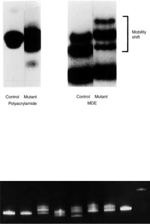
mutation detection electrophoresis. This gel has a somewhat hydrophobic character which |
|
|
|
|
||||||
alters the mobility of heteroduplexes selectively. Some move faster; most |
move slower. |
|
|
|
||||||
In good cases a single mismatched base in a 900 base pair duplex is sufficient to give an |
|
|
|
|||||||
easily detectable mobility shift. An example of the improved ability of |
MDE |
compared |
|
|
|
|
||||
with ordinary gel media to resolve heteroplexes from homoduplexes is shown in Figure |
|
|
|
|
||||||
13.17. A more complex example of the use of MDE is illustrated in Figure 13.18, where |
|
|
|
|||||||
it is clear that different heteroduplexes within the same basic DNA fragments show differ- |
|
|
|
|
||||||
ent mobilities. Thus, in principle, the method offers some promise of revealing, not just |
|
|
|
|||||||
that a heteroduplex is present but additional information about its characteristics. The ap- |
|
|
|
|||||||
peal of this method is that it is very easy to perform, since aside from the special proper- |
|
|
|
|||||||
ties of the gel, the electrophoretic procedures used are quite ordinary. It is also easy to an- |
|
|
|
|||||||
alyze many samples in parallel. However, the full generality of the method has yet to be |
|
|
|
|||||||
proved. For example, it would be good to know how the nature of the mismatch and its |
|
|
|
|||||||
location |
within the duplex affect the ability to |
detect |
it. Already |
we know |
that deletions |
|
|
|
||
lead to large mobility shifts, and DNA molecules with more than one heteroduplex region show very complex behavior. In general, a heteroduplex combination of a deletion and a separate, distant single-base mismatch leads to much larger mobility shifts than expected from the effects seen with the two mutations separately. The reason for this synergistic behavior is not currently understood.
A second electrophoretic method was originally developed by Leonard Lerman and his collaborators, and several variations on this general theme now exist. The original method
460 FINDING GENES AND MUTATIONS
|
(a ) |
(b ) |
|
|
|
Figure 13.17 |
An example of |
direct detection of heteroduplex DNA by electrophoresis. ( |
a ) |
On |
|
polyacrylamide. ( |
b ) On MDE gel. Provided by Avitech, Inc. |
|
|
|
|
was called denaturing gradient gel electrophoresis (DGGE). The basic idea behind the |
|
|
|||
method is illustrated in Figure 13.19. DGGE appears to be a general method capable of |
|
|
|||
detecting any mismatch in a DNA sequence that is not at the very end. An internal mis- |
|
|
|
||
match in a duplex leads to a substantial decrease in the thermodynamic stability; this is |
|
|
|||
manifested by a drop in the |
T m of the duplex (Fig. 13.19 |
a ). To test for mismatches, DNA |
|
|
|
fragments are electrophoresed in a |
gel through a gradient of increasing denaturant like |
|
|
||
urea, or a gradient of increasing temperature. At some critical point the section of the du- |
|
|
|||
plex containing |
the destabilizing |
mismatch reaches conditions above its local |
|
T m , and |
it |
Figure 13.18 Many different single mismatches can be distinguished by electrophoresis on MDE. Each lane is a different cystic fibrosis disease allele except for the left lane which is a normal allele, and shows no heteroduplex formation. Provided by Avitech, Inc.
HETERODUPLEX DETECTION |
461 |
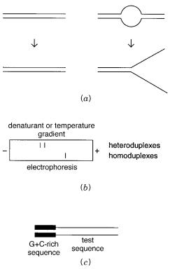
Figure 13.19 |
Denaturing gradient gel electrophoresis (DGGE) detection |
of |
heteroduplexes. ( |
a ) |
||||||||||||
Destabilization of a duplex by mismatching. ( |
|
|
|
|
b ) Electrophoresis in a temperature or denaturant gra- |
|
||||||||||
dient. ( c ) Use of a GC clamp to prevent strand separation in DGGE. |
|
|
|
|
|
|
|
|
||||||||
melts. The |
resulting |
Y -shaped |
structure (or one with a large internal loop) has little or no |
|
||||||||||||
electrophoretic mobility, and so the molecule |
is |
trapped in the |
gel |
near |
or |
at |
the |
site |
|
|||||||
where it melted (Fig. 13.19 |
|
b ). Thus from a single experiment one can determine not only |
|
|||||||||||||
whether heteroduplexes are present but |
also what kinds of mismatches were present, |
|
|
|||||||||||||
since most give characteristic and different shifts in |
|
|
|
|
|
T m . |
|
|
||||||||
It is important that the mismatch does not destabilize the duplex so much that the en- |
|
|||||||||||||||
tire structure melts into separate strands. These |
would |
still |
be free to migrate in |
the |
gel. |
|
||||||||||
To prevent this unwanted effect, a G |
|
|
|
|
C-rich sequence is usually placed at one end of the |
|
||||||||||
duplex to be tested. This is easily |
done |
by using PCR primers with an extra overhanging |
|
|||||||||||||
G C-rich sequence. The use of this so-called GC clamp (Fig. 13.19 |
|
|
|
|
c ) prevents complete |
|
||||||||||
melting under typical DGGE conditions. A major advantage of DGGE is its generality. |
|
|
||||||||||||||
Another advantage is that rather complex samples can be analyzed by running a gel com- |
|
|
|
|||||||||||||
posed of a restriction enzyme digest of a clone and then blotting it with particular probes. |
|
|||||||||||||||
A major disadvantage of DGGE is that specialized apparatus is needed for this method. |
|
|
|
|||||||||||||
A third electrophoretic method we |
will |
describe |
for |
detection |
of |
altered |
DNA se- |
|
||||||||
quences is also based on electrophoresis, |
and it takes advantage of the effects of altered |
|
||||||||||||||
DNA sequence on thermodynamic stability. |
However, in detail, this method is actually |
|
|
|||||||||||||
quite different from DGGE; it does not involve heteroduplexes. Called single-strand con- |
|
|
||||||||||||||
formational polymorphism (SSCP), the method is based on nondenaturing gel elec- |
|
|||||||||||||||
trophoresis |
of melted |
and rapidly |
cooled samples. Under |
these |
conditions |
individual |
|
|||||||||
462 FINDING GENES AND MUTATIONS
DNA strands fold back on themselves to form whatever combination of stems and loops (and other secondary structures, e.g., pseudoknots) that the particular DNA sequence al-
lows. Changes in even a single base can substantially alter the spectrum of secondary structures formed. RNA can be used instead of DNA to enhance the stability of secondary structure formation, and this apparently increases the fraction of heteroduplexes that can be detected. The use of MDE gels also enhances the resolution of SSCP. The results in a
typical SSCP analysis are complex. However, SSCP is serving as a very easy and sensitive method to detect a reasonable fraction of all possible heteroduplexes. Two variations
of SSCP have been described by Steven Sommer that increase the probability of detecting any mutation in the target. The first of these, called dideoxy fingerprinting (ddf ), is a hy-
brid between Sanger sequencing and SSCP (Sarkar et al., 1992). A Sanger ladder is produced with a single dideoxy pppN, and it is analyzed on a native polyacrylamide se-
quencing gel. In the second method, restriction endonuclease fingerprinting, the nucleases and the products from these digests are pooled and analyzed together by SSCP (Liu and
Sommer, 1995). |
|
A fourth electrophoretic method takes advantage of |
the power of automated fluores- |
cent DNA sequences. A mutation shows up as an unexpected |
peak. The sensitivity of the |
method, called orphan peak analysis (Hattori et al., 1993), is sufficient to allow multiple samples to be probed in each gel lane.
The final method we will mention for detecting altered DNA sequences is based on recent findings by Sergio Pena and coworkers (1994). In using short random DNA primers (RAPD; see Chapter 4) for PCR analysis of human DNA, they noted that the pattern of amplified bands seen was exquisitely sensitive to DNA sequence variations in the neigh-
borhood of the primers such that virtually all alleles tested led to a different, distinct pattern of amplified DNA lengths.
In current practice, faced with a gene to search for mutants, the simplest and most general existing method is probably to do both SSCP and MDE-heteroduplex analysis. The
real difficulty that remains is the size of many genes of interest. A typical 3- to 5-kb gene could be scanned in 5 to 10 pieces by selective PCR. In order to do this, however, one has to have available mRNA from the individual to be tested. This may not always be avail-
able. A further caveat is that some altered mRNAs may be selectively degraded in a cell if they are not functional. Thus a mutation may make itself invisible at the RNA level. The alternative is do the analysis at the DNA level. Here one can use PCR to look only at the exons. However, the difficulty is that some genes have 30 or more exons, and some exons can be very small. Given the large size of typical introns, each exon will have to be analyzed by a separate PCR reaction; thus the overall test becomes quite complicated.
DIAGNOSIS OF INFECTIOUS DISEASE
DNA sequence is proving to be quite useful in the diagnosis of the presence of infectious organisms. Usually a small bit of DNA sequence will suffice to indicate the presence of a virus, bacterium, protozoan, or fungus. Different species can be identified definitively, once their characteristic DNA sequences are known. The major problem in using DNA
analysis for detection of infectious agents is sensitivity; this is the same problem we encountered earlier in examining the prospects of DNA diagnosis for cancer. There may be
only a few copies of the DNA (or RNA, |
for some viruses) genome |
per |
organism. The |
number of infected cells (or the number |
of organisms free in the |
blood |
stream or other |