Berrar D. et al. - Practical Approach to Microarray Data Analysis

and it is useful to have a reference. For example, if a project decided that boosting (where the case weights in a data set are adjusted by the modelling algorithm to accentuate the hard-to-classify cases, which should improve the modelling of those cases) was ideal in a 5-class classification problem, and a year later a paper is published that points out shortcomings in such a use of boosting, then the project will have on record that it used the best information available at the time. The record should also make it more straightforward to repeat the analysis with a change in the boosting effect.

Going back to the example using the Golub et al. (1999) data set, the data will be thresholded, invariant genes removed, data normalised and clean at this point, and so modelling can begin. In an ideal world, the data could be run and the model(s) and results admired immediately, but in reality, once modelling begins, more data manipulation usually becomes necessary. It may be that the thresholding levels were too lax; for example instead of a lower limit of 20 and an upper of 1,600, 40 and 1,500 would be more appropriate. Again, keep track of the changes made and run the models again.

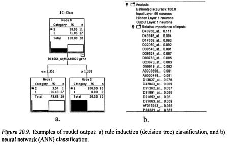
When results come back, interpretability of the results is very algorithmand software-dependent – some output is aesthetically pleasing, some takes a bit more effort. Examples of output represented in Figure 20.8. are presented in Figure 20.9. Rule Induction (Decision Tree) will present the gene(s) most significantly contributing to the discrimination between the classes (in this case two classes) and a Neural Network will present a list of relative importance to the discrimination. At this point, algorithms may be discarded or modified because they are not producing the detail of output that is required to address the business objective. If the analyst prefers the Decision Tree output format and interpretability, but the Decision Tree insists that just

one gene is doing all the discrimination, then perhaps a bagging approach to the decision tree would be more appropriate than relying on a single tree: bagging consists of select a series of subsets of genes to run against the class, and combine the resulting trees for an overall predictor (c.f. Chawla et al., 2001).

Nor is it necessary to just use one modelling technique in isolation; if two techniques are good classifiers but pick up different idiosyncrasies of the data, use the results of both to predict new cases. For example, accept the prediction of a particular class only in those cases where both modelling techniques agree, or accept the prediction of a class where at least one modelling technique accurately classifies (Figure 20.10.). The analyst can be creative with the use and combination of modelling techniques when searching for novel patterns.

Once the modelling techniques have been decided, a test design should accompany the selections, which describes the process by which the models will be tested for generalisability beyond the model-building data set and for success of the modelling exercise. Perhaps the most important aspect of the test design is deciding how the data are to be split into train and test samples, or use of cross-validation. In non-microarray data sets with many cases (more cases than variables) a train:test ratio can comfortably be up to 80:20. In microarray data a classification problem might be trying to discriminate among 4 classes spread across 40 cases. If 80% of the data are used to build the model, only 2 cases of each class will be left for testing the model’s generalisability. If it fails, it will be difficult to see where and why it failed, and how to improve the model. Whatever the ratio chosen, training and testing data are also often selected at random from the raw data set. In such small data sets, if 80% of the data are randomly selected as training, it is possible that only half of the classes would show up in the testing data set at all. Because of these dangers, cross-validation is rapidly picking up in popularity, and most modelling software supports cross-validation. Golub et al. (1999) describe the use of both types of validation in the classification analysis.

What will be the success criteria, or what sort of error rates will be used to determine the quality of model result? Answers will vary with data and modelling technique chosen. In a supervised modelling task, will classification rate be sufficient or will there be more weight put on the control of false positives? Using unsupervised techniques for class discovery, it may be more difficult to put a success or failure label on the results; looking for clusters of similarly expressing genes may be a good

start, but will that give you the answer that will fulfil project objectives – will the cheminformatics department be able to work with the cluster results or do they want further labelling of the clusters? Do the survival probabilities of the clusters make sense? Clustering techniques most often require human intervention, and an analysis of whether or not the clusters make sense will determine success. Again, as part of the documentation process, this subjective stage and possible ranges of results should be noted so that if an aberrant result comes up it can be rectified quickly and productivity is not lost.

If there are more than a few data sets to be analysed, generate a tick-list where completion of modelling steps for each data set can be noted, with space to document where the results can then be found. Having made it this far through the process, it is a good idea to ward against project collapse should the analyst be offered a better job elsewhere, hit the lecture circuit or decide not to return from a conference.

Algorithms, whether statistical or machine learning, generally have many parameters to tweak, and unless the analyst is trying to replicate a particular protocol, the parameters should be sensibly tweaked to see what happens. Some of the results will be rubbish, some will be useful, but all should be assessed as to whether or not they make sense. Iterate model building and assessment, throwing away models that are not useful or sensible, but keep track of what has been tried or it will inevitably be scrolled through again.

When the tick-list of models has been run through, there may be a series of models to rank if only the most successful of them are to be kept for use on future projects. This is where the previously-determined success criteria are used to greatest value, as it is easy to start hedging about the definition of success if the pet algorithm or freeware did not make into the top 5 hitlist. Having success criteria in place will also be a signal of when the parameter tweaking can be stopped and the process evaluated. Many projects simply stop when time or money runs out, while the actual analytical objectives had been long-satisfied and time has been lost in the drug discovery or publication process.

3.5Evaluation of Project Results

In the modelling phase, the individual models’ results are assessed for error and sensibility, and in this evaluation phase, the whole process is similarly assessed as outlined in Figure 20.11. Was there a bottleneck in the project – was it a problem with computers, people, data access? How can that be removed or decreased? How did the modelling perform relative to the Data Mining goal? Was a single model found that had the best classification rate? Or will a combination of models be used as the classification algorithm, with some preand post-model processing? What about the business objective? If the Data Mining goal has been achieved, then classification of new cases based on expression levels should be a trivial leap, as the data manipulation and cleaning required of the new cases, as well as the modelling techniques to be used, will be documented and possibly even automated by this point.

Did the project uncover results not directly related to the project objective that perhaps should redefine the objective or even define the next project? Results are a combination of models and findings, and peripheral findings can lead to both unexpected profits and attractive dead ducks. As such, it may be prudent to keep track of them, but perhaps save the pursuit of them for the next project.

3.6Deployment

Deployment is a very broad term. Essentially “doing something with the results”, it can cover anything from writing a one-off report to describe the analytical process, the writing of a thesis or publication, to informing an ongoing laboratory protocol, to the building of knowledge that will help take the field forward. Figure 20.12 shows the general steps that are taken when approaching the deployment phase of a project.

If the results or process are to be part of a laboratory protocol, once the desirable report (visualisation, modelling protocol or text/Powerpoint® output) is established, will it be a regular report? If so, the final process that was established through the above steps can be automated for re-use with similar data sets. The complexities of the data storage, cleaning and manipulation, model creation and comparison, and output-report production could be built into the automation to run with a minimum of human intervention, to save human patience for interpretation of the results. A production and maintenance schedule could be built to support the ongoing exertions, possibly with modelling-accuracy thresholds put in place to check the ongoing stability and validity of the model. In a production mode, alerts could be set up to warn when the models are no longer adequate for the data and should be replaced.

From the deployment phase of the Data Mining process, a summary of findings and how they relate to the original objectives – essentially a discussion section – would be a sensible addition to audit documentation. If you are the analyst that is offered a better job, it would be much nicer of you to leave a trail that your replacement could pick up on, and you would hope for the same from your new position.

The stream-programming concept of Data Mining shows its strengths at the evaluation and deployment stages, in a production environment as well as in cases of one-off analysis projects. The steps are self-documenting and visual, and the models quickly rebuilt using the same preand post-modelling processing steps as well as the same model parameters, as found with the traditional code programming. Visual programming permits a new analyst to pick up or repair an existing project with relatively small loss of productivity.

4.EPILOGUE

An analyst in the field of microarray data will be suffering the Red Queen syndrome for many years to come, as new algorithms and data manipulations are evolved, tested and discarded. If chips become less expensive, as usually happens with technology, then in the near future more experiments on a given project may be run and larger data sets generated, leading to yet another set of algorithms being appropriate for the peculiarities of microarray data. As such, establishing a framework for Data Mining that includes flexible boundaries and change, planning for the next steps to include testing of new algorithms or to tighten or loosen model success criteria, will prevent getting caught in the tulgey wood.

REFERENCES

Chawla N., Moore T., Bowyer K., Hall L., Springer C., Kegelmeyer P. (2001). Investigation of bagging-like effects and decision trees versus neural nets in protein secondary structure prediction. Workshop on Data Mining in Bioinformatics, KDD.

CRISP-DM: Cross-Industry Standard Process for Data Mining. Available at http://www.crispdm.org.

Golub T.R., Slonim D.K., Tamayo P., Huard C., Gaasenbeek M., Mesirov J.P., Coller H., Loh M., Downing J.R., Caligiuri M.A., Bloomfield C.D., Lander E.S. (1999). Molecular classification of cancer: class discovery and class prediction by gene expression monitoring. Science 286(5439):531-537.

(Data set available at: http://www-genome.wi.mit.edu/mpr/data_set_ALL_AML.html)

Moyle S., Jorge A. (2001) RAMSYS–A methodology for supporting rapid remote collaborative data mining projects. In Christophe Giraud-Carrier, Nada Lavrac, Steve Moyle, and Branko Kavsek, editors, Integrating Aspects of Data Mining, Decision Support and Meta-Learning: Internal SolEuNet Session, pp. 20-31. ECML/PKDD'01 workshop notes.