

Berrar D. et al. - Practical Approach to Microarray Data Analysis
.pdf344 |
Chapter 19 |
Schoeberl B., Eichler-Jonsson C., Gilles E.D., Muller G. (2002). Computational modeling of the dynamics of the MAP kinase cascade activated by surface and internalized EGF receptors. Nat Biotechnol. 20:370-375.
Selvin S. (1998). Modern Applied Biostatistical Methods: Using S-Plus. New York: Oxford University Press.
Sherlock G. (2001). Analysis of large-scale gene expression data. Brief Bioinform. 2:350-362.
Stewart J.E., Mangalam H., Zhou J. (2001). Open Source Software meets gene expression. Brief Bioinform. 2:319-328.
Tavazoie S., Hughes J.D., Campbell M.J., Cho R.J., Church G.M. (1999). Systematic determination of genetic network architecture. Nat Genet. 22:281–285.
Tomiuk S., Hofmann K. (2001). Microarray probe selection strategies. Brief Bioinform. 2:329-340.
Venables WN, Ripley BD. (1999). Modern Applied Statistics With S-Plus. New York: SpringerVerlag.
Wu T.D. (2001). Analysing gene expression data from DNA microarrays to identify candidate genes. J Pathol 195:53-65.
Yang Y.H., Buckley M.J., Speed T.P. (2001). Analysis of cDNA microarray images. Brief Bioinform 2:341-349.
Yang Y.H., Dudoit S., Luu P., Lin D.M., Peng V., Ngai J., Speed T.P. (2002). Normalization for cDNA microarray data: a robust composite method addressing single and multiple slide systematic variation. Nucleic Acids Res. 30:E15.
Chapter 20
MICROARRAY ANALYSIS AS A PROCESS
Susan Jensen
SPSS (UK) Ltd,St. Andrew’s House, West Street, Woking GU21 6EB, UK, e-mail: sjensen@spss.com
1.INTRODUCTION
Throughout this book, various pieces of the microarray data analysis puzzle are presented. Bringing the pieces together in such a way that the overall picture can be seen, interpreted and replicated is important, particularly where auditability of the process is important. In addition to auditability, results of the analysis are more likely to be satisfactory if there is a method to the apparent madness of the analysis. The term “Data Mining” is generally used for pattern discovery in large data sets, and Data Mining methodologies have sprung up as formalised versions of common sense that can be applied when approaching a large or complex analytical project.
Microarray data presents a particular brand of difficulty when manipulating and modelling the data as a result of the typical data structures therein. In most industries, the data can be extremely “long” but fairly “slim”
– millions of rows but perhaps tens or a few hundreds of columns. In most cases (with the usual number of exceptions), raw microarray data has tens of rows, where rows represent experiments, but thousands to tens of thousands of columns, each column representing a gene in the experiments.
In spite of the structural difference, the underlying approach to analysis of microarray retains similarities to the process of analysis of most datasets. This chapter sets out an illustrative example of a microarray Data Mining process, using examples and stepping through one of the methodologies.
2.DATA MINING METHODOLOGIES
As academic and industrial analysts began working with large data sets, different groups have created their own templates for the exploration and
346 Chapter 20
modelling process. A template ensures that the results of the experience can be replicated, as well as providing a framework for an analyst just beginning to approach a domain or a data set. It leaves an audit trail that may prevent repetition of fruitless quests, or allows new technology to intelligently explore results that were left as dead ends.
Published Data Mining methodologies have been produced by academic departments, software vendors and by independent special interest groups. There is general agreement on the basic steps comprising such a methodology, beginning with an understanding of the problem to be addressed, through to deploying the results and refining the question for the next round of analysis. Some methodologies concentrate solely on the work with the data, while others reinforce the importance of the context in which the project is undertaken, particularly in assessing modelling results.
Transparency of the Data Mining process is important for subsequent auditing and replication of the results, particularly in applications that face regulatory bodies. A very successful combination in Data Mining is a selfdocumenting analytical tool along with an established Data Mining methodology or process. There are several Data Mining tools (reviewed in Chapter 19) that implement a “visual programming” concept, where the steps taken in each phase of a methodology are documented and annotated by the creator, in the course of the project development. Examples of “visual programming” will be presented in later sections in this chapter. Importantly, though, any given methodology will generally be supported by whatever tool or set of tools is used for analysis, as the methodology is more a function of the user than the software.
An EU-funded project resulted in the Cross-Industry Standard Process for Data Mining (CRISP-DM; see http://www.crisp-dm.org). A consortium of some 200 representatives from industry, academia and software vendors set out to develop a common framework based upon the occasionally painful experiences that they had in early Data Mining activities. The idea was to improve both their own project management and to assist others tackling what could be an intimidating task, and the CRISP-DM document was published by the consortium in 1999.
Web searches and anecdotal information indicate that CRISP-DM is currently the single most widely-referenced Data Mining methodology, probably because the documentation is detailed, complete and is public access. CRISP-DM is visible as a project-management framework for consulting firms, and is actively supported by various Data Mining software vendors, such as NCR Teradata and SPSS, who were among the consortium participants. An example of extensions to CRISP-DM is in RAMSYS, (Moyle and Jorge, 1999 ), a methodology to improve remote collaboration
20. Microarray Analysis as a Process |
347 |
on Data Mining projects. RAMSYS was (and continues to be) developed by members of SolEUNet (Solomon European Virtual Enterprise).
Because of this visibility, I will use CRISP-DM as the framework for an example of working through the analysis or mining of microarray data in the subsequent section.
3.APPLICATION TO MICROARRAY ANALYSIS
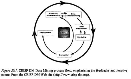
Whatever the origin of data, Data Mining tasks have unsurprising similarities, beginning with “what am I trying to do here?” and ending with “what have I done and what can I do with it?” In the following sections I will lay out the more formal version of those questions in a microarray data analysis project, in CRISP-DM steps (Figure 20.1). At the beginning of each section will be a general flow diagram outlining the sub-steps within each of the steps, to give a gentle introduction to that part of the process, to be fleshed out by application to microarray data.
For a detailed, step-by-step, industry-neutral guide on steps and tips in using CRISP-DM, the booklet can be downloaded from the Web site.
The approach of a Data Mining process will be familiar, roughly following the structure of a scientific paper. The process begins with the introduction of objectives and goals, to the methods and materials of data cleaning, preparation and modelling, to evaluation of results, concluding with discussion and deployment – where the results lead, what benefit gained, next steps to take.
348 |
Chapter 20 |
3.1Business Understanding
Analysis of microarray data is generally done with a specific objective or goal in mind, whether mapping active regions of a genome, classification of tissue types by response to a drug treatment, looking for gene expression patterns that might provide early indicators of a disease, and so on. This differs from a more classic Data Mining problem where someone is faced with a database and must think of appropriate, testable questions to ask of the data, in order to structure the information gained.
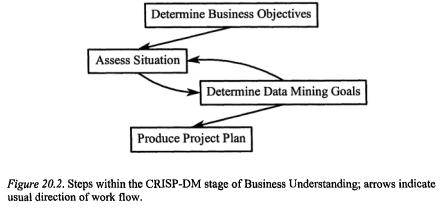
Because of the (likely) existing purpose in microarray data collection, the objectives (both the “business objective” and “Data Mining goal”; Figure 20.2.) of the analysis would likely already be determined. The fate of output of the project will obviously impact the goal: is it for scientific publication, is it part of an early drug discovery project where the results are to be fed to the cheminformatics department, or is it testing internal processes or equipment?
The public access leukemia gene expression data set described by Golub et al., (1999) can be used as a classification example throughout this process. The simplified and illustrative Data Mining process diagrams in this chapter were produced using the Clementine® Data Mining workbench.
Golub et al., (1999) describe one of the first attempts to classify cancer and tumour classes based solely on gene expression data, which is the clear business objective. The Data Mining goal was more specific: to use an initial collection of samples belonging to known classes to create a class predictor that could classify new, unknown samples (Golub et al,, 1999, p531). The next level of detail, algorithm selection and evaluation, is addressed in the modelling phase of the process (below), after developing an understanding of the data involved.
20. Microarray Analysis as a Process |
349 |
Within the business understanding phase, once the business objectives and Data Mining goal are stated, the next step would be to inventory the resources. How much time might be required, and will the people doing the analysis be available to complete the project? If not, are there others that could step in? What computing resources will be required, appropriate hardware and software for completing the analysis to satisfy the objective?
An idea of how long the analysis will take, including all the data manipulation required, is probably an unknown until you have been through it once. During that time, the analyst(s) may be interrupted to attend conferences, or follow up on other projects. Has time or contingency plans been built in to deal with the interruption?
If CRISP-DM were being used to help maintain an audit trail of the analysis, a project plan would be produced at this stage, with the inventory of resources, duration, inputs, outputs and dependencies of the project.
3.2Data Understanding
Data from microarray readers can be stored in text format, databases or Excel® spreadsheets, and may resemble that depicted in Table 20.1. The collation of data from several experiments may be done manually or via database appending processes. If the analysis involves combining several formats, such as expression data with clinical data, then at this stage the formats would be checked and any potential problems documented. For example, if the clinical data were originally collected for a different purpose, unique identifiers for individuals may not match between the files, and have to be reconciled in order to merge the data later.

350 |
Chapter 20 |
The audit trail would, in this section, document any problems encountered when locating, storing or accessing the data, for future reference, particularly if data quality becomes a question when results are returned from the analysis.
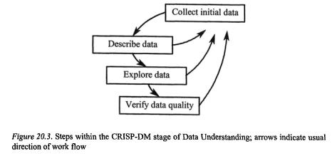
It is during this data understanding phase that the analyst would begin exploring the data, graphically analysing attributes, looking for possible relationships between variables, and checking the distribution of classes that might be predicted (c.f. Figure 20.3., depicted in Figure 20.4.). As with most data analyses, if there is an interesting pattern that comes out immediately, it is probably data contamination.
Time spent on examination of the data at this phase will pay off, as that is when data import or export errors are detected, and coding or naming problems are found and corrected (and documented). By the end of this phase, the analyst should have confidence in the quality and integrity of the data, and have a good understanding of the structure relative to the desired goal of the analysis.
20. Microarray Analysis as a Process |
351 |
3.3Data Preparation
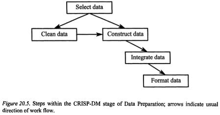
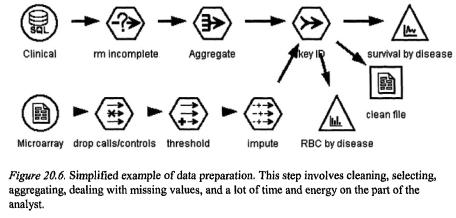
The objective of this step, as indicated in Figure 20.5., is to get all of the data ready to do the modelling. The data understanding and data preparation phases of any project usually represent about 80% of the work and about 90% of the tedium and frustration in dealing with data from any industry. Since techniques on data cleaning and imputation appropriate to the microarray analysis field are still evolving, much time may be spent in preparation in order to test, for example, the effects of different types of data normalisation or missing value imputation. There are several chapters in this book that detail various aspects of preparing microarray data for analysis, so I will speak in more general terms of selection, cleaning, and enriching the data.
Transposing the data, so that the experiments/subjects are in rows and genes in columns, may sound trivial but is one of the early and major hurdles for large data sets. Some steps in cleaning the data are easiest with genes as rows, others easiest with genes as columns. It is relatively simple to do the transposition in Excel provided that the end result will have only 255 genes or columns, which is unlikely with modern microarray data sets, which can hold up to 30,000 genes. Otherwise, it can be easily accomplished in a couple of steps in some Data Mining software, or through construction and implementation of repeated Perl scripts.
The preparation process generally begins with selection of the data to be used from the set collated. If Affymetrix chips are used, then removal of the calls and control fields is necessary for a clean analysis set. Expression levels may have registered at very low and very high levels, and the extremes are generally not meaningful, so deciding on upper and lower
352 |
Chapter 20 |
thresholds, and setting the outlier values to those thresholds will remove unnecessary noise. For example, it may be decided that values less than 20 and greater than 1,600 are not biologically meaningful; rather than simply exclude those values, the values less than 20 are replaced with 20, and those greater than 1,600 are replaced with the upper threshold of 1,600. Then the next step of finding and removing the invariant genes (i.e. those genes that are not differentially expressed) from the data will help to reduce the data set to a more meaningful set of genes (c.f. Figure 20.6.).
Decisions about standardising, centralising and/or normalising of the expression data, and imputation of missing values are discussed in previous chapters. If there are choices to be made among these data manipulation stages, it may be that several of the options will be implemented to test the results. The result may be that where there was one raw data file, there is now a developing library of several files with different permutations of the manipulation: e.g. data with overall-mean missing value imputation, data with group-mean imputation, data with k-nearest neighbour imputation, each of the imputed data sets with mean-centering, each of the imputed data sets with 0-1 centring, and so on.
Documentation of the library resulting from these decisions is a good idea, for the sanity of the analyst and to ensure that all the sets are treated similarly when the modelling phase is reached, as well as for assistance when dealing with queries about the results. Further manipulation, such as creation of new variables, tags indicating tissue class, categorisation of a target field into an active/inactive dichotomy or discretization of numeric fields, should also be documented for future reference and reproducibility.
If the microarray data are to be used in conjunction with clinical data, then the clinical data will be cleaned during this phase as well, so that the resulting formats will be compatible or at least comprehensible. Decisions
20. Microarray Analysis as a Process |
353 |
may have to be made on whether to aggregate, for example, lab exam results of the subjects by averaging, summing or taking the variance of the data for merging with the single line of gene expression data for each patient.
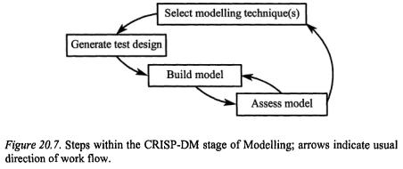
3.4Modelling
As mentioned in the last section, a single raw data file may, after the data preparation phase, have turned into a series of data sets that describe a matrix of normalisation and missing value replacement techniques, each of which to be analysed similarly for results comparison. It is often a good idea to be reminded of the goal of the project at this point to keep the analyses focused as you decide which modelling technique or techniques will be applied before embarking on the appropriate steps shown in Figure 20.7. For a given project, the list of algorithms should be narrowed to those appropriate and possible given the time, software and money allotted to the project.
There is an evolving variety of ways to reduce, classify, segment, discriminate, and cluster microarray data, as covered in Chapters 5 through 18 of this book. By the time you finish your project, more techniques, and tests on existing techniques, will have been published or presented at conferences. Because of these changes, it is very important to keep in mind (and preferably on paper) the assumptions, expected types of outcomes and limitations of each technique chosen to be used in the analysis, as well as how the outcome of each technique to be used relates to the Data Mining goal.
Documentation of why a particular modelling technique is used is also advisable because behaviours of techniques only become apparent after considerable use in different environments. As such, recommendations of when it is appropriate to use a given technique will likely change over time,