

Doicu A., Wriedt T., Eremin Y.A. Light scattering by systems of particles (OS 124, Springer, 2006
.pdf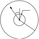
C.3 Computation of the Terms S11nn and S12nn |
293 |
Op |
|
2R |
S∞ |
|
θlp |
||
|
|
||
rlp |
SR |
|
|
|
Ol |
|
R∞
Fig. C.2. Illustration of the domain of integration bounded by the spherical surface SR and a sphere situated in the far-field region
|
|
2n + 1 |
|
|
|
Imm2 n = 32πR3jn |
|
|
ejKsz0l δmm Gn (Ks, ks, R) , |
(C.3) |
|
2 |
|||||
where
∞
Gn (Ks, ks, R) = [g (2Rx) − 1] h(1)n (2ksRx) jn (2KsRx) x2dx.
1
C.3 Computation of the Terms S11nn and S12nn
The terms S11nn |
and S12nn are given by |
|
|
|
|
|
|
|
|
|
|||||
|
|
|
∞ |
|
|
|
|
|
|
|
|
|
|
|
|
|
|
|
|
|
|
2n |
|
+ 1 |
|
|
|
|
|||
|
|
1 |
|
|
n |
|
|
|
|
1 |
|
|
|
||
|
|
S1nn |
= |
|
(−1) |
|
|
|
2 |
|
I1nn n , |
|
|||
|
|
|
n =0 |
|
|
|
|
|
|
|
|
|
|
|
|
|
|
|
∞ |
|
|
|
|
|
|
|
|
|
|
|
|
|
|
|
|
|
|
2n |
|
+ 1 |
|
|
|
|
|||
|
|
2 |
|
|
n |
|
|
|
|
2 |
|
|
|
||
|
|
S1nn |
= |
|
(−1) |
|
|
|
|
|
I1nn n , |
|
|||
|
|
|
|
|
|
2 |
|
|
|||||||
|
|
|
n =0 |
|
|
|
|
|
|
|
|
|
|
|
|
where |
|
|
|
|
|
|
|
|
|
|
|
|
|
|
|
I1 |
= |
π π1 |
(β)π1 |
(β) + τ 1(β)τ 1 |
(β) Pn |
|
(cos β) sin β dβ, |
|
|||||||
1nn n |
|
n |
n |
|
|
n |
|
n |
|
|
|
|
|
||
|
|
0 |
|
|
|
|
|
|
|
|
|
|
|
|
|
I12nn n |
= π πn1 (β)τn1 (β) + τn1(β)πn1 (β) Pn |
(cos β) sin β dβ. |
|
||||||||||||
|
|
0 |
|
|
|
|
|
|
|
|
|
|
|
|
|
To compute S11nn , we consider the function |
|
|
|
|
|
|
|
||||||||
|
|
fnn (β) = πn1 (β)πn1 (β) + τn1(β)τn1 (β) |
(C.4) |
||||||||||||

294 C Computational Aspects in E ective Medium Theory
for fixed values of the indices n and n . This function can be expanded in terms of Legendre polynomials
|
|
|
|
|
|
∞ |
|
|
|
|
|
|
|
|
|
|
|
|
|
|
|
|
|
|
|
|
|
||
|
fnn (β) = |
|
ann ,n Pn (cos β) , |
|
|
|
|
|
(C.5) |
||||||||||||||||||||
|
|
|
|
n =0 |
|
|
|
|
|
|
|
|
|
|
|
|
|
|
|
|
|
|
|
|
|
||||
where the expansion coe cients are given by |
|
|
|
|
|
|
|
|
|
|
|
|
|
|
|
||||||||||||||
ann ,n = π fnn (β)Pn |
(cos β) sin β dβ = I11nn n . |
||||||||||||||||||||||||||||
0 |
|
|
|
|
|
|
|
|
|
|
|
|
|
|
|
|
|
|
|
|
|
|
|
|
|
|
|
|
|
Using the special value of the Legendre polynomial at β = π, |
|
|
|||||||||||||||||||||||||||
|
|
|
|
|
|
|
|
|
|
|
|
|
|
|
|
|
|
|
|
|
|
|
|
|
|||||
|
Pn (cos π) = ( |
|
|
|
1)n |
|
2n + 1 |
, |
|
|
|
|
|
|
|
||||||||||||||
|
|
|
|
|
|
2 |
|
|
|
|
|
|
|
|
|
||||||||||||||
|
|
|
|
|
|
|
|
− |
|
|
|
|
|
|
|
|
|
|
|
|
|
|
|
|
|||||
we see that (C.5) leads to |
|
|
|
|
|
|
|
|
|
|
|
|
|
|
|
|
|
|
|
|
|
|
|
|
|
|
|
|
|
|
∞ |
|
|
|
|
|
|
|
|
|
|
|
|
|
|
|
|
|
|
|
|
|
|
||||||
|
|
|
|
2n + 1 |
|
|
|
|
|
|
|
|
|
|
|
|
|
||||||||||||
|
( 1) |
n |
|
|
|
|
|
|
|
1 |
|
n |
|
|
= |
|
|
1 |
|
. |
|
||||||||
fnn (π) = |
|
|
|
|
|
|
|
|
|
|
|
I1nn |
|
|
|
|
1nn |
|
|
||||||||||
|
n =0 |
|
− |
|
|
|
|
|
|
|
|
2 |
|
|
|
|
|
|
|
|
|
S |
|
|
|
|
|||
|
|
|
|
|
|
|
|
|
|
|
|
|
|
|
|
|
|
|
|
|
|
|
|
|
|
|
|
|
|
On the other hand, since |
|
|
|
|
|
|
|
|
|
|
|
|
|
|
|
|
|
|
|
|
|
|
|
|
|
|
|
|
|
πn1 (π) = |
(−1)n−1 |
|
|
|
|
|
, |
|
|
|
|
||||||||||||||||||
n(n + 1) (2n + 1) |
|
|
|
|
|||||||||||||||||||||||||
|
|
|
|
|
|
|
|
|
|
|
|||||||||||||||||||
|
|
|
2√2 |
|
|
|
|
|
|
|
|
|
|
|
|
|
|
|
|
|
|
|
|
|
|||||
τ 1(π) = |
(−1)n |
|
|
|
|
. |
|
|
|
|
|
|
|||||||||||||||||
n(n + 1) (2n + 1) |
|
|
|
|
|
|
|||||||||||||||||||||||
|
n |
|
√ |
|
|
|
|
|
|
|
|
|
|
|
|
|
|
|
|
|
|
|
|
|
|
|
|
|
|
|
|
2 |
2 |
|
|
|
|
|
|
|
|
|
|
|
|
|
|
|
|
|
|
|
|
|
|
|
|||
(C.4) implies that |
|
|
|
|
|
|
|
|
|
|
|
|
|
|
|
|
|
|
|
|
|
|
|
|
|
|
|
|
|
fnn (π) = snn = |
(−1)n+n |
|
|
|
|
|
(C.6) |
||||||||||||||||||||||
n(n + 1) (2n + 1) |
n (n |
+ 1) (2n + 1) |
|||||||||||||||||||||||||||
4 |
|
|
|
|
|
|
|
|
|
|
|
|
|
|
|
|
|
|
|
|
|
|
|
|
|
|
|
|
|
and therefore,
S11nn = snn .
Analogously, we find that
S12nn = −snn .

D
Completeness
of Vector Spherical Wave Functions
The completeness and linear independence of the systems of radiating and regular vector spherical wave functions on closed surfaces have been established by Doicu et al. [49]. In this appendix we prove the completeness and linear independence of the regular and radiating vector spherical wave functions on two enclosing surfaces. A similar result has been given by Aydin and Hizal [5] for both the regular and radiating vector spherical wave functions with nonzero divergence, i.e., the solutions to the vector Helmholtz equation.
Before formulating the boundary-value problem for the Maxwell equations we introduce some normed spaces which are relevant in electromagnetic scattering theory. With S being the boundary of a domain Di we denote by [39, 40]
Ctan(S) = {a/a C(S), n · a = 0}
the space of all continuous tangential fields and by
Ctan0,α(S) = a/a C0,α(S), n · a = 0 , 0 < α ≤ 1 ,
the space of all uniformly H¨older continuous tangential fields equipped with the supremum norm and the H¨older norm, respectively. The space of uniformly H¨older continuous tangential fields with uniformly H¨older continuous surface divergence ( s) is defined as
0,α |
|
0,α |
(S), s · a C |
0,α |
(S) |
|
Ctan,d |
(S) = |
a/a Ctan |
|
, 0 < α ≤ 1 , |
while the space of square integrable tangential fields is introduced as
L2tan(S) = a/a L2(S), n · a = 0 .
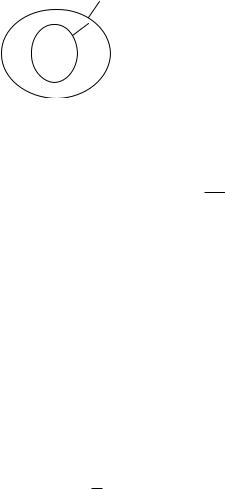
Now, let S1 and S2 be two closed surfaces of class C2, with S1 enclosing S2 (Fig. D.1). Let the doubly connected domain between S1 and S2 be denoted by Di,1, the domain interior to S2 by Di,2, the domain interior to S1 by Di,
296 D Completeness of Vector Spherical Wave Functions
n1 
n2 
εi,µi O 
Di,2 |
S2 |
S1 |
|
Di,1 |
|
|
Ds |
Fig. D.1. The closed surfaces S1 and S2
and the domain exterior to S1 by Ds. We assume that the origin is in Di,2, and denote by n1 and n2 the outward normal unit vectors√to S1 and S2, respectively. The wave number in the domain Di,1 is ki = k0 εiµi, where k0 is the wave number in free space, and εi and µi are the relative permittivity and permeability of the domain Di,1. We introduce the product spaces
Ctan(S1,2) = Ctan(S1) × Ctan(S2),
C0tan,α(S1,2) = Ctan0,α(S1) × Ctan0,α(S2) ,
C0tan,α,d(S1,2) = Ctan0,α,d(S1) × Ctan0,α,d(S2) ,
L2tan(S1,2) = L2tan(S1) × L2tan(S2),
and define the scalar product in L2tan(S1,2) by
- x1 |
|
y1 |
. |
x2 |
, |
y2 |
= x1, y1 2,S1 + x2, y2 2,S2 . |
|
|
|
2,S1,2 |
The Maxwell boundary-value problem for the doubly connected domain Di,1 has the following formulation.
Find a solution Ei, Hi C1(Di,1) ∩ C(Di,1) to the Maxwell equations in
Di,1
× Ei = jk0µiHi , × Hi = −jk0εiEi,
satisfying the boundary conditions
n1 × Ei = f 1 |
on |
S1 , |
n2 × Ei = f 2 |
on |
S2 , |
where f 1 and f 2 are given tangential vector fields.
Denoting by σ(Di,1) the spectrum of eigenvalues of the Maxwell boundaryvalue problem, we assume that for f 1 Ctan0,α,d(S1) and f 2 Ctan0,α,d(S2), both

D Completeness of Vector Spherical Wave Functions |
297 |
Ei and Hi belong to C0,α(Di,1), and for ki / σ(Di,1), the Maxwell boundaryvalue problem possesses an unique solution.
Theorem 1. Consider Di,1 a bounded domain of class C2 with boundaries S1 and S2. Define the vector potentials
A1(r) = a1(r )g(ki, r, r )dS(r ) ,
S1
A2(r) = a2(r )g(ki, r, r )dS(r )
S2
for a1 L2tan(S1) and a2 L2tan(S2), assume ki / σ(Di,1) and
× × A1 + × × A2 = 0
in Ds and Di,2. Then a1 0 on S1 (a1 vanishes almost everywhere on S1), and a2 0 on S2.
Proof. Defining the electromagnetic fields
j
E = k0εi ( × × A1 + × × A2) ,
j
H = −k0µi × E = × A1 + × A2,
passing to the boundary along a normal direction and using the jump relations for the curl of a vector potential with square integrable density [49], we find that
0 = lim |
n1 × H (· + hn1 (·)) |
|
|
|
|
|
||||||||
h 0+ |
|
|
|
|
|
|||||||||
→ |
|
|
|
|
|
|
|
|
|
|
|
|
|
|
! |
|
|
|
|
|
|
|
|
|
|
1 |
|
" |
|
− n1 × × |
S1 a1(r )g(ki, ·, r )dS(r ) + |
|
a1 |
|
||||||||||
2 |
|
|||||||||||||
|
|
|
|
|
a (r )g(k , |
, r )dS(r ) |
= |
|
|
|
||||
n |
× × |
|
|
= |
|
|
|
|||||||
− 1 |
|
|
|
2 |
|
i · |
|
= |
|
|
|
|||
|
|
|
|
S2 |
|
|
|
|
|
=2,S1 |
|
|||
and |
|
|
|
|
|
|
|
|
|
|
|
|
|
|
0 = h 0+ |
|
n |
2 × H |
· − |
hn |
2 |
· |
|
|
|
|
|
||
lim |
|
|
( |
|
|
|
( )) |
|
|
|
|
|
||
→ |
|
|
|
|
|
|
|
|
|
|
|
|
|
|
! |
|
|
|
|
|
|
|
|
|
|
1 |
|
" |
|
− n2 × × |
S2 a2(r )g(ki, ·, r )dS(r ) − |
|
a2 |
|
||||||||||
2 |
|
|||||||||||||
|
|
|
|
|
a (r )g(k , |
, r )dS(r ) |
= |
|
|
|
||||
n |
× × |
|
|
= . |
|
|||||||||
− 2 |
|
|
|
1 |
|
i · |
|
= |
|
|
|
|||
|
|
|
|
S1 |
|
|
|
|
|
=2,S2 |
|
|||

298 D Completeness of Vector Spherical Wave Functions
Defining the operators |
|
|
|
|
|
(M11a) (r) = n1 (r) × × S1 a(r )g(ki, r, r )dS(r ) , r S1, |
||
|
|
|
(M12a) (r) = n1(r) × × S2 a(r )g(ki, r, r )dS(r ) , r S1 , |
||
and |
|
|
|
|
|
(M21a) (r) = n2(r) × × S1 a(r )g(ki, r, r )dS(r ) , r S2 , |
||
|
|
|
(M22a) (r) = n2(r) × × a(r )g(ki, r, r )dS(r ) , r S2 ,
S2
we obtain
1
2 I + M11 a1 + M12a2 = 0,
almost everywhere on S1, and
|
1 |
|
|
−M21a1 + |
|
I − M22 |
a2 = 0, |
2 |
almost everywhere on S2. Note that M11 and M22 are the singular magnetic operators on the surfaces S1 and S2, respectively, while M12 and M21 are nonsingular operators. In compact operator form, we have
|
|
|
a + Ka = 0, |
|
|
|
|
|
|
|
||
where |
|
|
|
|
|
|
|
|
|
|
|
|
a = |
a1 |
|
|
|
2 |
11 |
2 |
M |
12 |
|
||
|
|
and = |
M |
|
− |
|
|
. |
||||
|
a2 |
|
K |
|
− M |
|
M |
22 |
|
|||
|
|
|
2 |
21 |
2 |
|
|
|
||||
The above integral equation is a Fredholm integral equation of the second kind,
and according to Mikhlin [161] we find that a a0 Ctan(S1,2). Noticing that the operator K map Ctan(S1,2) into C0tan,α(S1,2) and C0tan,α(S1,2) into C0tan,α,d(S1,2),
0,α |
|
|
a10 |
|
we see that a a0 Ctan,d |
(S1,2), where a0 |
= |
a20 |
. The properties of the |
vector potentials with uniformly H¨older continuous densities, then yields E, H C0,α(Di,1). The jump relations for the double curl of the vector potentials A1 and A2 [49], give n1 × E− = 0 on S1, and n2 × E+ = 0 on S2. Therefore, E and H solve the homogeneous Maxwell boundary-value problem, and since ki / σ(Di,1), it follows that E = H = 0 in Di,1. Finally, from the jump relations (for continuous densities)
n1 × H+ − n1 × H− = a10 = 0,

D Completeness of Vector Spherical Wave Functions |
299 |
and
n2 × H+ − n2 × H− = a20 = 0,
we obtain a1 0 on S1, and a2 0 on S2.
The following theorems state the completeness and linear independence of the system of regular and radiating spherical vector wave functions on two enclosing surfaces.
Theorem 2. Let S1 and S2 be two closed surfaces of class C2, with S1 enclosing S2, and let n1 and n2 be the outward normal unit vectors to S1 and S2, respectively. The system of vector functions
# $ n1 × M mn3 |
% , |
$ n1 × N mn3 |
% , |
$ n1 × M mn1 |
% , |
$ n1 × N mn1 |
% , |
n2 × M mn3 |
|
n2 × N mn3 |
|
n2 × M mn1 |
|
n2 × N mn1 |
|
|
|
|
|
+ |
|
|
|
n = 1, 2, . . . , m = −n, . . . , n/ki / σ (Di,1)
is complete in L2tan(S1,2).
Proof. It is su cient to show that for a = |
a1 |
|
2 |
|||
a2 |
|
Ltan(S1,2), the set of |
||||
closure relations |
|
|
|
|
|
|
S1 a1 · n1 × M mn3 |
dS + S2 a2 · n2 × M mn3 dS = 0, |
|||||
|
3 |
|
|
|
|
3 |
S1 a1 |
· n1 × N mn dS + |
S2 a2 |
· n2 × N mn dS = 0, |
|||
and |
|
|
|
|
|
|
S1 a1 · n1 × M mn1 |
dS + S2 a2 · n2 × M mn1 dS = 0, |
|||||
|
1 |
|
|
|
|
1 |
S1 a1 |
· n1 × N mn dS + |
S2 a2 |
· n2 × N mn dS = 0 |
|||
for n = 1, 2, . . ., and m = −n, . . . , n, yields a1 0 on S1, and a2 0 on S2. As in the proof of Theorem 1, we consider the vector potentials A1 and A2 with densities a1 = n1 × a1, and a2 = n2 × a2, respectively, and define the vector field
j
E = k0εi ( × × A1 + × × A2).
Restricting r to lies inside a sphere enclosed in S2 and using the vector spheri-
cal wave expansion of the dyad gI, we see that the first set of closure relations gives E = 0 in Di,2. Analogously, but restricting r to lies outside a sphere enclosing S1, we deduce that the second set of closure relations yields E = 0 in Ds. Theorem 1 can now be used to conclude.

300 D Completeness of Vector Spherical Wave Functions
Theorem 3. Under the same assumptions as in Theorem 2, the system of vector functions
# $ n1 × M mn3 |
% , |
$ n1 × N mn3 |
% , |
$ n1 × M mn1 |
% , |
$ n1 × N mn1 |
% , |
n2 × M mn3 |
|
n2 × N mn3 |
|
n2 × M mn1 |
|
n2 × N mn1 |
|
|
|
|
|
+ |
|
|
|
n = 1, 2, . . . , m = −n, . . . , n/ki / σ (Di,1)
is linearly independent in L2tan(S1,2).
Proof. We need to show that for any Nrank, the relations
Nrank |
n |
$ |
3 |
% |
$ |
3 |
% |
|
αmn |
|
n1 × M mn |
+ βmn |
n1 × N mn |
|
|
||
n=1 m=−n |
|
n2 × M mn3 |
|
n2 × N mn3 |
|
|
||
+γmn |
$ n1 × M mn1 % + δmn $ n1 × N mn1 |
% = 0 , |
$ on |
S1 % |
||||
|
n2 × M mn1 |
n2 × N mn1 |
|
on |
S2 |
|||
give αmn = βmn = γmn = δmn = 0, for n = 1, 2, . . . , Nrank and m = −n, . . . , n. Defining the electromagnetic field
Nrank n
E = αmnM 3mn + βmnN 3mn + γmnM 1mn + δmnN 1mn, n=1 m=−n
we see that n1 × E = 0 on S1 and n2 × E = 0 on S2. The uniqueness of the Maxwell boundary-value problem then gives E = 0 in Di,1, and since E is an analytic function we deduce that E = 0 in Di −{0}. Using the representations for the vector spherical wave functions M 1mn,3 and N 1mn,3 in terms of vector spherical harmonincs mmn and nmn, and the fact that the system of vector spherical harmonics is orthogonal on the unit sphere, we obtain
αmnh(1)n (kir) + γmnjn (kir) = 0,
βmn kirh(1)n (kir) + δmn [kirjn (kir)] = 0,
for r > 0. Taking into account the expressions of the spherical Bessel and Hankel functions for small value of the argument
jn(x) = |
|
|
xn |
1 + O x2 |
|
|||
|
|
|
|
|||||
|
|
(2n + 1)!! |
|
|||||
and |
|
|
|
|
|
|
|
|
h(1) |
(x) = |
− |
j |
(2n − 1)!! |
1 + O x2 |
, |
||
n |
|
|
xn+1 |
|
||||