Vankka J. - Digital Synthesizers and Transmitters for Software Radio (2000)(en)

can be realized as M + 1 parallel FIR filters of length N having the coefficient values cm(i). The transfer functions of these filters are given by

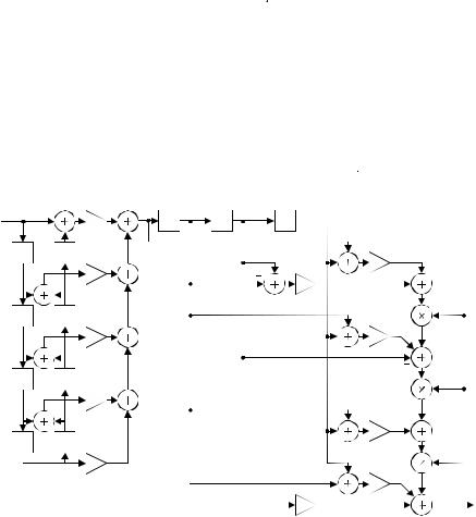
The interpolant y(kTout) is obtained by multiplying the output samples of the parallel filters vm(n) by ( k)m for m = 0, 1,..., M. The Farrow structure realization of the interpolator described above is depicted in Figure 12-5. This efficient structure is implemented using the Horner's method [Väl95]

M

¦vm (n)(µk )m v0 (n) + [v1 (n) + [v2 (n) + + [vM −1 (n) + vM (n)µk ]µk ]µk ]µk (12.10)

m= 0

The number of the FIR filter coefficients in the Farrow structure is N(M + 1). These coefficients are fixed and the multiplications can be efficiently implemented as, for example, Canonic Signed Digit taps described in Section 11.6. In addition to these, M multiplications by the fractional interval k are needed. This results in the total number of multiplications M+N(M + 1). This is a maximal number; usually some of the coefficients are 0 or ±1 and they do not have to be implemented, or two coefficients may have the same value and thus the hardware can be shared [Väl95]. The unit delay elements of the filters Cm(z) can also be shared in order to reduce the amount of hardware.

Some modifications to the Farrow structure are presented in [Ves99] and [Väl95]. The modification in [Ves99] results in the symmetric or antisymmetric impulse responses of the FIR filters Cm(z) in the Farrow structure if

ha(t) is symmetrical, i.e. if they are linear-phase Type II or Type IV filters.

x(m)

cM(N/2)

Z-1

cM(N/2 -1)

C2(z) C1 (z)

Z-1

cM(-N/2+1)

Figure 12-5 Farrow structure for a polynomial-based interpolator.

length 9 [Ves95]. The B-spline interpolators have a better stopband attenuation than the Lagrange interpolators of the same degree [Ves99]. Actually, the stopband attenuation of the Lagrange interpolator cannot be greatly improved by increasing the degree of interpolation. The main problems of both the Lagrange and B-spline interpolations are a wide transition band and fairly poor frequency selectivity for the wideband signals.

A better frequency-domain behavior for the wideband signals can be achieved by using a frequency-domain approach. The polynomial coefficients of the impulse response ha(t) can be optimized directly in the frequency domain. These methods have usually at least three design parameters, which makes them more flexible compared to the time-domain methods with only one design parameter. These parameters include the length of the filter N, the degree of the interpolation M, which is not tied to the length of the filter as is the case with the time-domain methods, and the passband edge

p . Some methods also allow the definition of the passband and stopband regions. In [Ves96a], [Far98], [Laa96] and [Ves98], for example, several frequency domain design methods are discussed. All these interpolators are mentioned as offering a better frequency response for the wideband signals than the filters based on the Lagrange or B-spline interpolations [Ves99]. An interpolator designed using the method presented in [Ves96a] is taken here as an example. It is referred to here as the Vesma-Saramäki interpolator (see Figure 12-7). The output instant for the interpolant y(kTout) in Figure 12-7 is

hp(2) = 0,124355653

hp(3) = -0,33320997

hp(4) = 0,008928334

Figure 12-6 The structure of the cubic B-spline interpolator

controlled by (2 k 1), and not by k like for the Lagrange and B-spline interpolators. The filter coefficients in Figure 12-7 were designed so that the frequency-domain error function is minimized in the minimax sense [Ves96a], [Ves00].

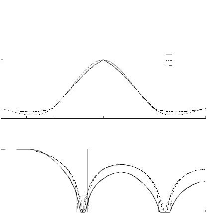
The Computational Complexity and the maximum level of the attenuated images of the cubic Lagrange (see Figure 16-7), cubic B-spline (see Figure 12-6) and Vesma-Saramäki (see Figure 12-7) interpolators are compared in Table 12-2. The interpolators are used as a resampler in GSM/EDGE/WCDMA modulator in Figure 16-6. The image rejection specification is more than 75 dB in WCDMA mode. The interpolation filter specifications in Table 12-2 are as follows: the passband is [0 0.0625Fs], the stopbands are [0.9375 Fs, 1,0625 Fs] and [1.9375 Fs, 2,0625 Fs], the maximum passband deviation is 0.05 dB, and the minimum stopband attenuation is 75 dB. The magnitude responses of the cubic Lagrange (see Figure 16-7), cubic B-spline (see Figure 12-6) and Vesma-Saramäki (see Figure 12-7) interpolators are depicted in Figure 12-8. One important property of the interpolator, when using it as a sampling rate converter, is the phase linearity. The continuous time impulse responses of the cubic Lagrange, cubic B-spline and Vesma-Saramäki interpolators are symmetric around t = 0 (see Figure 12-8) and thus they have linear phase. The elements of the prefilter are added to the number of elements of the B-spline interpolator in Table 12-2. The number of operations only gives an overview, because they depend on the implementation of the interpolator and thus there is no unique way to calculate

0.1147

-0.0386

0.1157

y

Figure 12-7 The structure of the Vesma-Saramäki interpolator.

them. Scaling by a constant is considered a fairly simple operation that can be performed using the multiplierless coefficients described in Section 11.6. The passband ripple is here the maximum value of the frequency response minus unity. The values in Table 12-2 indicate that the cubic Lagrange interpolator is the most appropriate method of these with a sufficient performance and an efficient realization. It is therefore used in Figure 16-6.

Even though the results in some articles, in [Ves96b], for example, indicate that the frequency domain approaches are better in performance and in computational complexity, this was not the result in this case. The values in Table 12-2 indicate that the time-domain approach, the B-spline interpolation and the Lagrange interpolation give performance similar to the frequency domain approach Vesma-Saramäki interpolation. A reason for this discrepancy in the results is that, in this case, the sampling rate is increased before the re-sampler by an integer ratio in Figure 16-6 and so the ratio of the signal bandwidth to the sampling rate is smaller (0.0625Fs).

Some other polynomial interpolation methods worthy of a mention are the piece-wise parabolic explained and used in [Eru93], [Cho01], for example, and the use of the trigonometric functions as interpolation functions in, for example, [Fu99]. The disadvantage of the interpolation filters based on

IMPULSE RESPONSES

1.2

0.8

0.6

0.4

0.2 0

-0.2-2 -1.5 -1 -0.5 0 0.5 1 1.5 2 t/TS

FREQUENCY RESPONSES

0 -20 -40

-60

-80

-100

Frequency/FS

Figure 12-8 Impulse and magnitude responses of cubic Lagrange (see Figure 16-7), cubic B- spline (see Figure 12-6) and Vesma-Saramäki (see Figure 12-7) interpolators.

Figure 12-9 Output of the NCO for control word 0.35.

the trigonometric interpolation is that they do not offer good frequency selectivity for wideband signals, i.e. for signals with the highest baseband frequency component close to half the sampling rate [Ves99]. In [Sne99], an average of the overlapping interval of multiple polynomials fitted to different input samples is used for the interpolation. This way lower-order polynomials can be used to calculate the interpolant using the same number of input samples that is used by one higher-order polynomial. This approach is mentioned to provide a better aliasing rejection with only slightly more complex coefficient calculation than using only one lower-order polynomial.

12.5 Calculation of Fractional Interval k Using

NCO

As shown by (12.3), in case of a polynomial-based interpolation, there is no need to calculate the polynomial coefficients cm(i) on-line. The only variables in the interpolation (12.2) are the fractional interval k [0,1) and the index n of the input samples. The approximations of these variables can be calculated using a numerically controlled oscillator (NCO) [Gar93]. The

where the positive ∆φ is the NCO control word and mod[] denotes the modulus operation. The NCO is clocked with the output sampling rate Fout of the interpolator. The output of the NCO, which is a positive fraction, will be incremented by an amount ∆φ at every Tout seconds and the register will

overflow every 1/∆φ clock ticks, on average. The control word ∆φ can be calculated using the equation

Fout

Figure 12-9 shows the output η of the NCO for a control word ∆φ = 0.35. When an overflow occurs, the MSB of the binary NCO output word (k) switches from the state '1' to the state '0'. As mentioned, this happens on average at intervals

sampling clock of the interpolator (it must be inverted when a rising edge logic is used). This clock controls the shift registers in the Farrow structure shown in Figure 12-5 and therefore takes care of the index n. Because the output of the NCO can change only at the clock tick, (12.13) holds only on average, introducing some jitter to the clock derived from the MSB [Gar93].

From the triangles in Figure 12-9 the following equation can be derived

By substituting Equation (12.12) and (12.1) into the denominator, it follows

NCO

k [7:0]

clk clk

Figure 12-10. NCO with the synchronizer used for fractional interval calculation and clock

generation.

actly, the accuracy of the approximation depends on the word length of the NCO [Int01]. The maximum error of the control word ∆φ is half the LSB. This error can be corrected by using a timing recovery loop and adding the derived error signal to the control word ∆φ

12.5.1 Synchronization of Resampling NCO

The infinite word length of the digital control word ǻφbin makes it not always possible to have a binary control word representing the ideal ǻφ exactly. This means that the input registers of the interpolator are sampling either a little too fast or a little too slow. The error of the closest binary control word is

and j is the number of bits in the binary control word. The error will occur in the MSB used as the sampling clock for the interpolator after ncyc = 2-1/ɽǻφ clock cycles and after

seconds. For 32-bit NCO with εǻφ = 0.00000000009313 and Fout = 80MHz, the error will occur after 67.1 s. This is a rather long time and if the operation of the interpolator can be interrupted and the device reset before the error occurs, there is no need for compensation. Of course, according to (12.17) and (12.18) the error will occur even less frequently if the word length of the control word is increased. Naturally there are also cases where ǻφbin = ǻφ and then (12.17) equals zero and no compensation is needed. In the devices that require continuous-time operation, the error due to the infinite length control word causes sampling errors. To prevent this, the NCO

has to be synchronized to the input data. This can be done by varying the control word between values that are a little too large and a little too small, such that on average the control word is equivalent to the accurate value. A phase comparator can be used to compare the phase of the generated clock and the reference clock that implies the input data sample periods. If the generated clock has been drifted due to a too small control word, a compensation value is added to the control word and the phase of the generated clock drifts back to the optimum phase. The compensation word can be chosen so small that it has a negligible effect on the much shorter fractional interval k and on interpolation result. At smallest, the compensation word might be no larger the size of the LSB of the control word. For example, if ǻφ = 0.4 and j = 32, we get ǻφbin = 0.39999999990687, and by adding one LSB we get ǻφbin + LSB = 0.40000000013970. Such a synchronizer is actually a simple phase locked loop, where the loop filter is of the first order. The block diagram of the NCO with the synchronizer is depicted in Figure 12-10.

After the device is reset, the phase of the generated clock can be far from the optimum. In this case, with a very small compensation word the drifting to optimum phase can take a very long time, depending on how accurate the frequency control word is. To prevent this long initialization time, we can use a larger compensation value for fast drifting and change the value to the

Figure 12-12. Phase difference of the reference clock and the generated clock when synchronizer is in use (solid line) and not in use (dashed line).

smaller one after the coarse synchronization is found. This kind of synchronization technique changes the phase drifting introduced by the inaccuracy of control word to a phase jitter, which can be tolerated without sampling errors if the overall interpolation ratio of the system is large enough.

The jitter is of the order of the output clock cycle (12.19), so the larger the interpolation ratio, the better the jitter can be handled, since the jitter is proportionally smaller compared to the input clock cycle.

The implementation of the phase compare block in Figure 12-10 is based on two digital saturating counters running at the output sampling frequency. A block diagram of the phase compare block is shown in Figure 12-11. The counters measure the phase difference of the reference clock and the generated clock in both directions. The result is given in output sampling periods. Because the counters have to be able to measure the worst case phase difference in output clock cycles, the number of bits needed in the counters is determined by the largest overall interpolation ratio for which the system is intended. The smaller of the measured differences is selected as the compensation word. The selection of the counter also defines the direction of the phase difference and therefore the sign of the compensation word. When the

Figure 12-13. Output of 3rd-order Lagrangian interpolator when synchronizer is in use (solid line) and not in use (dashed line).