


Chapter 3 - Fundamental PLC Programming
Chapter 3 - Fundamental PLC Programming
3-1. Objectives
Upon completion of this chapter, you will know
”how to convert a simple electrical ladder diagram to a PLC program.
”the difference between physical components and program components.
”why using a PLC saves on the number of physical components.
”how to construct disagreement and majority circuits.
”how to construct special purpose logic in a PLC program, such as the oscillator, gated oscillator, sealing contact, and the always-on and always-off contacts.
3-2. Introduction
When writing programs for PLCs, it is beneficial to have a background in ladder diagramming for machine controls. This is basically the material that was covered in Chapter 1 of this text. The reason for this is that at a fundamental level, ladder logic programs for PLCs are very similar to electrical ladder diagrams. This is no coincidence.
The engineers that developed the PLC programming language were sensitive to the fact that most engineers, technicians and electricians who work with electrical machines on a day-to-day basis will be familiar with this method of representing control logic. This would allow someone new to PLCs, but familiar with control diagrams, to be able to adapt very quickly to the programming language. It is likely that PLC programming language is one of the easiest programming languages to learn.
In this chapter, we will take the foundation knowledge learned in Chapter 1 and use it to build an understanding of PLC programming. The programming method used in this chapter will be the graphical method, which uses schematic symbols for relay coils and contacts. In a later chapter we will discuss a second method of programming PLCs which is the mnemonic language method.
3-3. Physical Components vs. Program Components
When learning PLC programming, one of the most difficult concepts to grasp is the difference between physical components and program components. We will be connecting physical components (switches, lights, relays, etc.) to the external terminals on a PLC. Then when we program the PLC, any physical components connected to the PLC will be represented in the program as program components. A programming component
3-1
Chapter 3 - Fundamental PLC Programming
will not have the same reference designator as the physical component, but can have the same name. As an example, consider a N/O pushbutton switch S1 named START. If we connect this to input 001 of a PLC, then when we program the PLC, the START switch will become a N/O relay contact with reference designator IN001 and the name START. As another example, of we connect a RUN lamp L1 to output 003 on the PLC, then in the program, the lamp will be represented by a relay coil with reference designator OUT003 and name RUN (or, if desired, “RUN LAMP”).
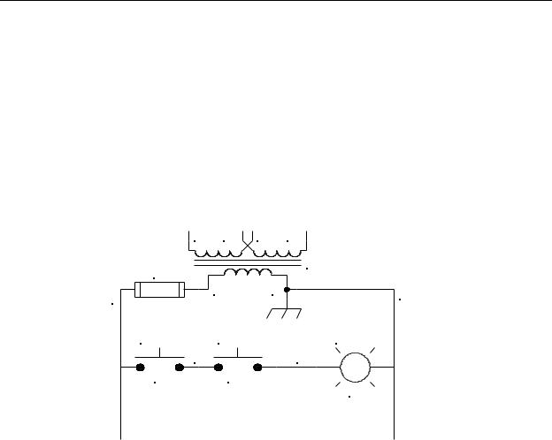
As a programming example, consider the simple AND circuit shown in Figure 3-1 consisting of two momentary pushbuttons in series operating a lamp. Although it would be very uneconomical to implement a circuit this simple using a PLC, for this example we will do so.
H1 |
H3 |
H2 |
|
H4 |
F1 |
|
|
|
T1 |
|
|
|
|
|
2 |
X1 |
|
X2 |
1 |
|
|
|
||
|
|
|
|
|
SWITCH1 |
SWITCH2 |
|
LAMP1 |
|
3 |
|
|
|
4 |
PB1 |
PB2 |
|
|
L1 |
|
|
|
|
|
Figure 3-1 - AND Ladder Diagram
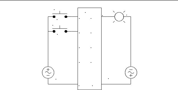
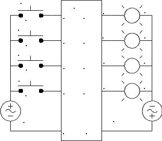
When we convert a circuit to run on a PLC, we first remove the components from the original circuit and wire them to the PLC as shown in Figure 3-2. One major difference in this circuit is that the two switches are no longer wired in series. Instead, each one is wired to a separate input on the PLC. As we will see later, the two switches will be connected in series in the PLC program. By providing each switch with a separate input to the PLC, we gain the maximum amount of flexibility. In other words, by connecting them to the PLC in this fashion, we can “wire” them in software any way we wish.
The two 120V control voltage sources are actually the same source (i.e., the control transformer secondary voltage). They are shown separately in this figure to make it easier to see how the inputs and output are connected to the PLC, and how each is powered.
3-2
Chapter 3 - Fundamental PLC Programming
SWITCH1 |
PLC |
|
|
|
L1 |
||
PB1 |
IN1 |
OUT1 LAMP1 |
|
|
|
|
|
SWITCH2 |
|
|
|
PB2 |
IN2 |
OUT2 |
|
|
|
|
|
|
IN3 |
OUT3 |
|
|
IN4 |
OUT4 |
|
120V |
|
120V |
|
CONTROL |
|
CONTROL |
|
VOLTAGE |
|
VOLTAGE |
|
|
COM |
COM |
|
Figure 3-2 - PLC Wiring Diagram for implementation of Figure 3-1
Once we know how the external components are wired to the PLC, we can then write our program. In this case we need to connect the two switches in series. However, once the signals are inside the PLC, they are assigned new reference designators which are determined by the respective terminal on the PLC. Since SWITCH1 is connected to IN1, it will be called IN1 in our program. Likewise, SWITCH2 will become IN2 in our program. Also, since LAMP1 is connected to OUT1 on the PLC, it will be called relay
OUT1 in our program. Our program to control LAMP1 is shown in Figure 3-3.
| |
IN1 |
IN2 |
OUT1 |
1 |
---| | |
-------| |--------------------------------------------------------- |
(OUT)| |
| |
|
|
|
| |
|
|
|
Figure 3-3 - AND PLC Program
The appearance of the PLC program may look a bit unusual. This is because this ladder rung was drawn by a computer using ASCII characters instead of graphic characters. Notice that the rails are drawn with vertical line characters, the conductors are hyphens, and the coil of OUT1 is made of two parentheses. Also, notice that the right rail is all but missing. Many programs used to write and edit PLC ladder programs leave out the rails. This particular program (TRiLOGI by TRi International Pte. Ltd.) Leaves out the right rail, but puts in the left one with a rung number next to each rung.
3-3
Chapter 3 - Fundamental PLC Programming
When the program shown in Figure 3-3 is run, the PLC first updates the input image register by storing the values of the inputs on terminals IN1 and IN2 (it stores a one if an input is on, and a zero if it is off). Then it solves the ladder diagram according to the way it is drawn and based on the contents of the input image register. For our program, if both
IN1 and IN2 are on, it turns on OUT1 in the output image register (careful, it does NOT turn on the output terminal yet!). Then, when it is completed solving the entire program, it performs another update. This update transfers the contents of the output image register (the most recent results of solving the ladder program) to the output terminals. This turns on terminal OUT1 which turns on the lamp LAMP1. At the same time that it transfers the contents of the output image register to the output terminals, it also transfers the logical values on the input terminals to the input image register. Now it is ready to solve the ladder again.
For an operation this simple, this is a lot of trouble and expense. However, as we add to our program, we will begin to see how a PLC can economize not only on wiring, but on the complexity (and cost) of external components.
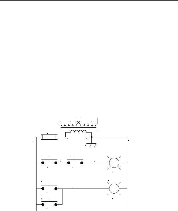
Next, we will add another lamp that switches on when either SWITCH1 or SWITCH2 are on. If we were to add this circuit to our electrical diagram in Figure 3-1, we would have the circuit shown in Figure 3-4
H1 |
H3 |
H2 |
H4 |
|
F1 |
|
|
T1 |
|
|
|
|
|
|
2 |
X1 |
|
X2 |
1 |
|
|
|
||
|
|
|
|
|
SWITCH1 |
SWITCH2 |
|
LAMP1 |
|
3 |
|
|
4 |
|
PB1 |
PB2 |
|
|
L1 |
|
|
|
|
|
SWITCH1 |
|
|
|
LAMP2 |
|
|
|
|
|
|
5 |
|
|
|
PB1 |
|
|
|
|
SWITCH2 |
|
|
|
L2 |
PB2 |
|
|
|
|
Figure 3-4 - OR Circuit |
|
|||
3-4
Chapter 3 - Fundamental PLC Programming
Notice that to add this circuit to our existing circuit, we had to add additional contacts to the switches PB1 and PB2. Obviously, this raises the cost of the switches. However, when doing this on a PLC, it is much easier and less costly.
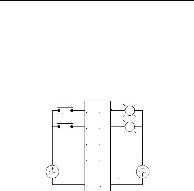
The PLC wiring diagram to implement both the AND and OR circuits is shown in Figure 3-5. Notice here that the only change we’ve made to the circuit is to add LAMP2 to the PLC output OUT2. Since the SWTICH1 and SWITCH2 signals are already available inside the PLC via inputs IN1 and IN2, it is not necessary to bring them into the PLC again.
This is because of one unique and very economical feature of PLC programming. Once an input signal is brought into the PLC for use by the program, you may use as many contacts of the input as you wish, and the contacts may be of either N/O or N/C polarity. This reduces the cost because, even though our program will require more than one contact of IN1 and IN2, each of the actual switches that generate these inputs, PB1 and PB2, only need to have a single N/O contact.
SWITCH1 |
PLC |
|
|
|
L1 |
||
PB1 |
IN1 |
OUT1 LAMP1 |
|
|
|
|
|
SWITCH2 |
|
|
|
|
IN2 |
LAMP2 |
L2 |
PB2 |
OUT2 |
|
|
|
|
|
|
|
IN3 |
OUT3 |
|
|
IN4 |
OUT4 |
|
120V |
|
120V |
|
CONTROL |
|
CONTROL |
|
VOLTAGE |
|
VOLTAGE |
|
|
COM |
COM |
|
Figure 3-5 - PLC Wiring Diagram to Add
SWITCH2 and LAMP2
Now that we have the inputs and outputs connected, we can write the program. We do this by simply adding to the program the additional rung that we need to perform the OR operation. This is shown in Figure 3-6. Keep in mind that other than the additional lamp and the time it takes to add the additional program, this additional OR feature costs nothing.
3-5
|
|
|
Chapter 3 - Fundamental PLC Programming |
|
| |
IN1 |
IN2 |
OUT1 |
|
1--- |
| | |
-------| |--------------------------------------------------------- |
(OUT)| |
|
| |
|
|
|
|
| |
|
|
|
|
| |
IN1 |
|
OUT2 |
|
| |
|
|||
2--- |
| | |
-------------------------------------------------------------------| |
(OUT)| |
|
| |
IN2 |
|
|
|
|--- |
| |--- |
+ |
|
|
| |
|
|
|
|
| |
|
|
|
|
|
|
|
Figure 3-6 - PLC Program with Added OR Rung |
|
Next, we will add AND-OR and OR-AND functions to out PLC. For this, we will need two more switches, SWITCH3 and SWITCH4, and two more lamps, LAMP3 and LAMP4. Figure 3-7 shows the addition of these switches and lamps.
SWITCH1 |
PLC |
|
|
|
L1 |
||
PB1 |
IN1 |
OUT1 LAMP1 |
|
|
|
|
|
SWITCH2 |
|
|
|
|
IN2 |
LAMP2 |
L2 |
PB2 |
OUT2 |
|
|
|
|
|
|
SWITCH3 |
|
|
|
|
|
LAMP3 |
L3 |
PB3 |
IN3 |
OUT3 |
|
SWITCH4 |
|
|
|
|
IN4 |
LAMP4 |
L4 |
PB4 |
OUT4 |
|
|
|
|
|
|
120V |
|
120V |
|
CONTROL |
|
CONTROL |
|
VOLTAGE |
|
VOLTAGE |
|
|
COM |
COM |
|
Figure 3-7 - PLC Wiring Diagram Adding
Switches PB3 and PB4 and Lamps L3 & L4.
Once the connection scheme for these components is known, we can add the additional programming required to implement the AND-OR and OR-AND functions. This is shown in Figure 3-8.
3-6