


Chapter 8 - Discrete Position Sensors
Chapter 8 - Discrete Position Sensors
8-1. Objectives
Upon completion of this chapter, you will know
”the difference between a discrete sensor and an analog sensor.
”the theory of operation of inductive, capacitive, ultrasonic, and optical proximity sensors.
”which types of proximity sensors are best suited for particular applications.
”how to select and specify proximity sensors.
8-2. Introduction
Generally, when a PLC is designed into a machine control system, it is not simply put into an open loop system. This would be a system in which the PLC provides outputs, but never “looks” to see if the machine is responding to those outputs. Instead, PLCs are generally put into a closed loop system. This is a system in which the PLC monitors the performance of the machine and provides the appropriate outputs at the correct times to make the machine operate properly, efficiently, and intelligently. In order to provide the
PLC with a sense of what is happening within the machine, we use sensors.
In a way, a limit switch is a sensor. The switch senses when its actuator is being pressed and sends an electrical signal to the PLC input. The limit switch provides the PLC with a crude sense of touch. However, in many cases, the PLC needs to sense something more sophisticated than a switch actuation. For these applications, sensors are available that can sense nearly any parameter that may occur in a machine environment.
This text has by no means a comprehensive coverage of all the currently available sensor technology. Because of uses of lasers, chroma recognition, image recognition, and other newer technologies, the state of sensor sophistication and variety of sensors is constantly evolving. Because of this rapid evolution, even experienced designers find it difficult to keep pace with sensor technology. Generally, machine controls and automation designers rely on manufacturer’s sales representatives to keep them abreast of newly developing technologies. In many cases a visit by a sales representative to view and discuss the potential sensor application will result in suggestions, catalogs, on-site demonstrations of sample units, and, if necessary, phone contact with a vendor’s field engineer to further discuss the application. This network of sales representatives and applications engineers should not be ignored by the designer - they are a valuable resource. In fact, most of the material covered in this and subsequent chapters is provided by manufacturer’s sales representatives.
8-1
Chapter 8 - Discrete Position Sensors
8-3. Sensor Output Classification
Fundamentally, sensor outputs are classified into two categories - discrete
(sometimes called digital, logic, or bang-bang) and proportional (sometimes called analog). Discrete sensors provide a single logical output (a zero or one). For example, a thermostat that operates the heating and air conditioning in a home is a discrete sensor. When the room temperature is below the thermostat’s setpoint, it outputs a zero, and when the temperature rises so that it is above the setpoint, the thermostat switches on and provides a logical one output. It is important to remember that discrete sensors do not provide information about the current value of the parameter being sensed. It only decides if the parameter being sensed is above or below the setpoint. Again, using the thermostat example, if the thermostat is set for 70 degrees and it is off, all that can be concluded is that he room temperature is below 70 degrees. The room temperature could be 69 degrees, minus 69 degrees, or any other value below 70 degrees, and the thermostat will give the same logical zero output.
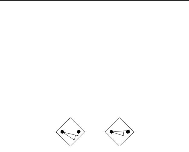
The schematic symbol for the discrete sensor is shown as a limit switch in a diamond shaped box. This is shown in Figure 8-1. Since this is a generic designation, we usually write a short description of the sensor type next to the symbol.
(a) |
(b) |
Figure 8-1 - Sensor Schematic Symbol
Proportional sensors, on the other hand, provide an analog output. The output may be a voltage, current, resistance, or even a digital word containing a discrete value. In any case, the sensor measures the value of the parameter, converts it to a signal that is proportional to the value, and outputs that value. When proportional sensors are used with
PLCs, they are generally connected to analog inputs on the PLC instead of the digital inputs. An example of a proportional sensor is the fluid level sending unit in the fuel tank of an automobile that sends a signal to operate the fuel level gage. This is generally a potentiometer in the fuel tank that is operated by a float. As the fuel level changes, the float adjusts the potentiometer and its resistance changes. The fuel gage is nothing more than an ohmmeter that indicates the resistance of the fuel level sensor.
For discrete sensors, there are two types of outputs, the NPN or sinking output, and the PNP or sourcing output. The NPN or sinking output has an output circuit that functions similar to a TTL open collector output. It can be regarded as an NPN bipolar transistor with
8-2
Chapter 8 - Discrete Position Sensors
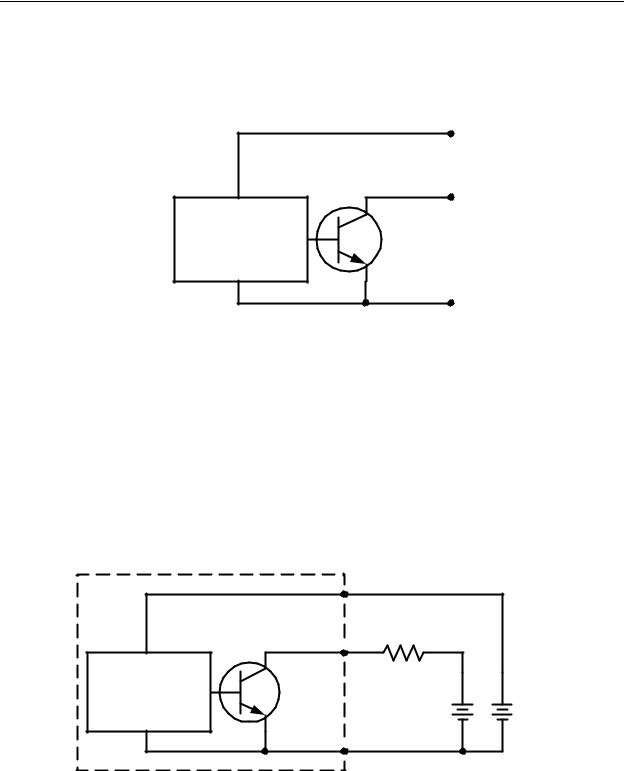
a grounded emitter and an uncommitted collector, as shown in Figure 8-2. In reality, this output circuit could be composed of an actual NPN transistor, an FET, an opto-isolator, or even a relay or switch contact. However, no matter how the output circuitry is composed, in operation it presents either an open circuit or a grounded line for its two output logical signals.
Vcc
Output
Proximity
Sensor
Circuitry
Gnd
Figure 8-2 - Sensor with NPN Output
Although at first this may seem rather convoluted and confusing, there is a specific application for an output circuit such as this. Since one of the logical states of the output is an open circuit, it can be used to drive loads that are outside of the power supply range of the sensor. This means that it is capable of operating a load that is being powered from a separate power supply, as shown in Figure 8-3. For example, it is relatively easy to have
a sensor that requires a +10 vdc power supply (Vsensor) operate a load operating from +24 vdc (Vload). Of course, it is also permissible to operate the NON output from the same power supply as the sensor. Typically, sensors with NPN outputs are capable of controlling
load voltages up to 30 vdc. The power supply for the load can be any voltage between zero and the maximum collector voltage specified for the output transistor.
Sensor
Vcc
Output Load
Proximity
Sensor Vload Vsensor
Circuitry
Gnd
Figure 8-3 - NPN Sensor Load Connection
8-3
Chapter 8 - Discrete Position Sensors
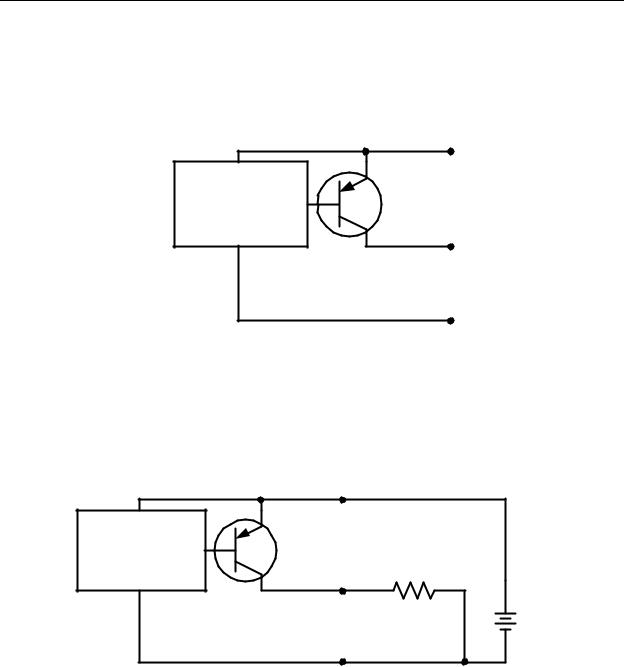
The PNP or sourcing output, has output logic levels that switch between the sensor’s power supply voltage and an open circuit. In this case, as illustrated in Figure 8-4, the PNP output transistor has the emitter connected to Vcc and the collector uncommitted. When the output is connected to a grounded load, the transistor will cause the load voltage to be either zero (when the transistor is off) or approximately Vcc (when the transistor is on).
Vcc
Proximity
Sensor
Circuitry
Output
Gnd
Figure 8-4 - Sensor with PNP Output
This is ideal for supplying loads that have power supply requirements that are the same as that of the sensor, and one of the two connection wires of the load is already connected to ground. Notice in Figure 8-5 that this allows a simpler design because only one power supply is needed. However, the disadvantage in this type of circuit is that the sensor and the load must be selected so that they operate from the same supply voltage.
Vcc
Proximity
Sensor
Circuitry
Output Load
Vcc
Gnd
Figure 8-5 - PNP Sensor Load Connection
8-4