Chapter 10 - Closed Loop and PID Control

the proportional and derivative gain constants, kp and kd. However, the designer should take caution in doing so because the electrical voltage and current transients, and mechanical force transients can become excessive with potentially damaging results.

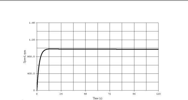
Figure 10-13 - DC Motor Speed Control with High kp and Moderate Derivative Gain kd

Although the transient response of our motor control system has been vastly improved, the offset is still present. By increasing the derivative constant kd, we eliminated the overshoot and hunting, but this had no effect on the offset. As indicated in Figure 10-13, the proportional and derivative functions nearly drove the motor speed to the proper value, but then the speed began to droop. As we will investigate next, in order to reduce this offset, the integral function must be used.

Based on the results of our investigations of the derivative function in a PID closed loop control system, we can make the following general conclusion:

In a properly tuned PID control system, the derivative function improves the transient response of the system by reducing overshoot and hunting. A byproduct of the derivative function is the ability to increase the proportional gain with increased stability, reduced settling time, and reduced offset.

10-7. Integral Function

A true integral is defined as the graphical area contained in the space bordered by a plot of the function and the horizontal axis. Integrals are cumulative; that is, as time passes, the integral keeps a running sum of the area outlined by the function being integrated. To illustrate this, we will take the integral of the pulse function shown in

10-13

Chapter 10 - Closed Loop and PID Control

Figure 10-14a. This function switches from 0 to 2 at time t = 0, switches back to 0 at time t = 1 second, then at time t = 2 seconds switches to -3, and finally back to 0 at t = 3 seconds. The integral of this waveform is shown in Figure 10-14b.

Figure 10-14 - Accumulated Area (Integral) of a Pulse Waveform

When the input waveform in Figure 10-14a begins at time t = 0 we will assume that the integral starting value is zero. As time increases from 0 to 1 second, the area under the waveform increases, which is indicated by the rising waveform in Figure 10-14b. At 1 second when the waveform switches off, the total accumulated area is 2. Since the input is zero between t = 1 and t = 2, no additional area is accumulated. Therefore, the accumulated area remains at 2 as indicated by the output waveform in Figure 10-14b between t = 1 and t = 2. At t = 2, the input switches to -3, and the integral begins adding negative area to the total. This causes the output waveform to go in the negative direction.

Since the area under the negative pulse of the input waveform between t = 2 and t = 3 is

-3, the output waveform will decrease by 3 during the same time period.

Notice that the output waveform in Figure 10-14b ends at a value of -1. This is the total accumulated area of the input waveform in Figure 10-14a during the time period t = 0 to t = 4. In fact, we can determine the total accumulated area at any time by reading the value of the integral in Figure 10-14b at the desired time. For example, the total accumulated area at t = 0.5 second is +1, and the total accumulated area at t = 2.5 seconds is +0.5.

For the example waveform in Figure 10-14a, the integral process seems simple. However, as with the derivative, if we wish to take the exact integral of a waveform that is nonlinear, such as a sine wave, the problem becomes more complicated and requires the use of calculus. For a control system (such as a PLC) this would be a heavy mathematical burden. So to lessen the burden, we instead have the PLC sample the input waveform at short evenly spaced intervals and calculate the area by multiplying the height (the

10-14

Chapter 10 - Closed Loop and PID Control

In a closed loop system, whenever there is an offset in the response, there will be a non zero error signal. This is because the PV and the SP are not equal. Since the integral function input is connected to the same error signal as the derivative function, the integral will begin to sum the error over time. For large offsets, the integral will accumulate rapidly and its output will increase quickly. For smaller offsets, the integral output will change more slowly. However, note that as long as the offset is non-zero, the integral output will be changing in the direction that will reduce the offset. Therefore, in a closed loop PID control system we can reduce the offset to near zero by increasing the integral gain constant, ki to some positive value.

Therefore, we will now attempt to reduce the offset in our motor speed control example to zero by activating the integral function. Figure 10-16 shows the result of increasing ki. Note that the transient response has changed little, but after settling, the offset is now zero.

Figure 10-16 - DC Motor Speed Control with

High kp, Moderate Derivative Gain kd, and

Low Integral Gain ki.

It is not advisable to make the integral gain constant ki excessively high. Doing so causes the integral and proportion functions to begin working against each other which will make the system more unstable. Systems with excessive values of ki will exhibit overshoot and hunting, and may oscillate.

To summarize the purpose of the integral function, we can now make the following general statement.

In a closed loop PID system, the integral function accumulates the system error over time and corrects the error to be zero or nearly zero.

10-16