

Chapter 10 - Closed Loop and PID Control
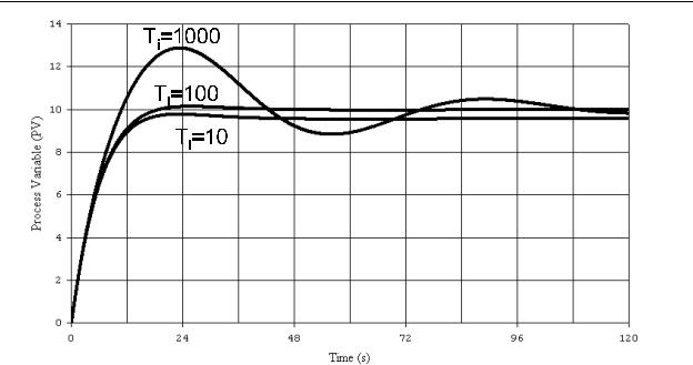
Figure 10-19 - Ti Adjustment
5.Once the initial PID tuning is complete, the designer may now make further adjustments to the three tuning constants if desired. From this starting point the
designer has the option to vary the proportional gain kp over a wide range. This can be done to obtain a faster response to a setpoint change. If the system is to operate with varying loads, it is extremely important to test it for system stability under all load conditions.
10-6. The Ziegler-Nichols Tuning Method
The Ziegler-Nichols tuning method (also called the ZN method) was developed in
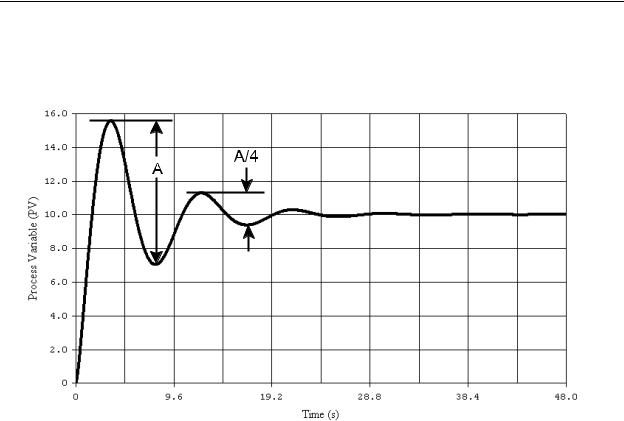
1942 by two employees of Taylor Instrument Companies of Rochester, New York. J.G. Ziegler and N.B. Nichols proposed that consistent and approximate tuning of any closed loop PID control system could be achieved by a mathematical process that involved measuring the response of the system to a change in the setpoint and then performing a few simple calculations. This tuning method results in an overshoot response which is acceptable for many control systems, and at least a good starting point for the others. If the desired response is to have less overshoot or no overshoot, some additional tuning will be required. The target amount of overshoot for the ZN method is to have the peak-to- peak amplitude of each cycle of overshoot be 1/4 of the previous amplitude, as illustrated
10-22
Chapter 10 - Closed Loop and PID Control
in Figure 10-20. Hence, the ZN method is sometimes called the 1/4 wave decay method.
Although it is unlikely that the ZN tuning method will achieve and exact 1/4 wave decay in the system response, the results will be a stable system, and the tuning will be approximated so that the system designer can do the final tweaking using an “adjust and observe” method.
Figure 10-20 - 1/4 Wave Decay
The main advantage in using the ZN tuning method is that all three tuning constants kp, Td, and Ti, are pre-calculated and input to the system at the same time. It does not require any trial and error to achieve initial tuning. The chief disadvantage in using ZN tuning is that in order to obtain the system’s characteristic data to make the calculations, the system must be operated either closed loop in an oscillating condition, or open loop. We shall investigate both approaches.
Oscillation Method
Using the oscillation method, we will be determining two machine parameters called the ultimate gain ku and the ultimate period Tu. Using these, we will calculate kd, Ti and Td.
1.Initialize all PID constants to zero. Power-up the machine and the closed loop control system.
2.Increase the proportional gain kp to the minimum value that will cause the system to oscillate. This must be a sustained oscillation, i.e., the amplitude of the oscillation must be neither increasing nor decreasing. It may be necessary to make changes in the setpoint to induce oscillation.
10-23
Chapter 10 - Closed Loop and PID Control
3.Record the value of kp as the ultimate gain ku.
4.Measure the period of the oscillation waveform. The period is the time (in seconds) for it to complete one cycle of oscillation. This period is the ultimate period Tu.
5.Shut down the system and readjust the PID constants to the following values:
kp = 0.6 ku Ti = 0.5 Tu
Td = 0.125 Tu
As an example, we will apply the Ziegler-Nichols oscillation tuning method to our example motor speed control system that was used earlier in this chapter. First, with all of the gains set to zero, we increase the proportional gain kp to the point where the process variable is a sustained oscillation. This is shown in Figure 10-21 and occurs at kp = 505 (which is the ultimate gain ku).
Figure 10-21 - ZN Tuning Method OScillation
It is then determined from this graph that, since it makes 10 cycles of oscillation in 90 seconds, the period of oscillation and the ultimate period Tu is approximately 9 seconds. Next we use the previously define equations to calculate the three gain constants.
kp = 0.6 ku = (0.6)(505) = 303 Ti = 0.5 Tu = (0.5)(9) = 4.5
Td = 0.125 Tu = (0.125)(9) = 1.125
We then input these gain constants into the system and test the response with a setpoint change from zero to 1000, which is shown in Figure 10-22.
10-24
Chapter 10 - Closed Loop and PID Control
Figure 10-22 - Final Result of ZN Tuning, Oscillation Method
Open Loop Method
For the open loop method, we will be determining three machine parameters called the deadtime L, the process time constant T, and the process gain K. Using these, we will calculate kd, Ti and Td. These measurements will be made with the system in an open loop unity gain configuration; that is, with the process variable PV (the feedback) open circuited, the proportional gain set to 1 (kd = 1), and the integral and derivative gains set to zero
(Ti = Td = 0). The tuning steps are as follows.
1.Input a known change the setpoint. This should be a step change.
2.Using a chart recorder, record a graph of the process variable PV with respect to time with time zero being the instant that the step input is applied.
3.On the graph, draw three intersecting lines. First, draw a line that is tangential to the steepest part of the rising waveform. Second, draw a horizontal line on the left of the graph at an amplitude equal to the initial value of the PV until it intersects the first line. Third, draw a horizontal line on the right of the graph at an amplitude equal to the final value of the PV until it intersects the first line.
4.Find the deadtime L as the time from zero to the point where the first and second lines intersect.
5.Find the process time constant T as the time difference between the points where the first line intersects the second and third.
10-25
Chapter 10 - Closed Loop and PID Control
6.Find the process gain K as the percent of the PV with respect to the CV (the PV divided by the CV).
7.Shut down the system and readjust the PID constants to the following values:
kp = 1.5T/(KL)
Ti = 2.5L Td = 0.4L
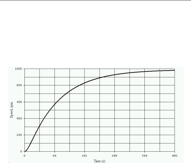
As an example, we will apply the Ziegler-Nichols open loop tuning method to our example motor speed control system that was used earlier in this chapter. Figure 10-23 shows the open loop response of the system with a SP change of zero to 1000.
Figure 10-23 - ZN Tuning Open Loop Response
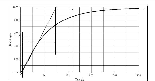
Next we will add the three specified lines to the graph as shown in Figure 10-24.
10-26
Chapter 10 - Closed Loop and PID Control
L |
|
T |
PV Change |
Figure 10-24 - System Open Loop Step Response
From the graph we can see that the deadband L is approximately 7 seconds, the process time constant T is 135 seconds, and the change in the setpoint is 980, which results in a process gain K of 0.98. Next we substitute these constants into our previous equations.
kp = 1.5T/(KL) = (1.5 x 135)/(0.98 x 7) = 29.5 Ti = 2.5L = (2.5)(7) = 17.5
Td = 0.4L = (0.4)(7) = 2.8
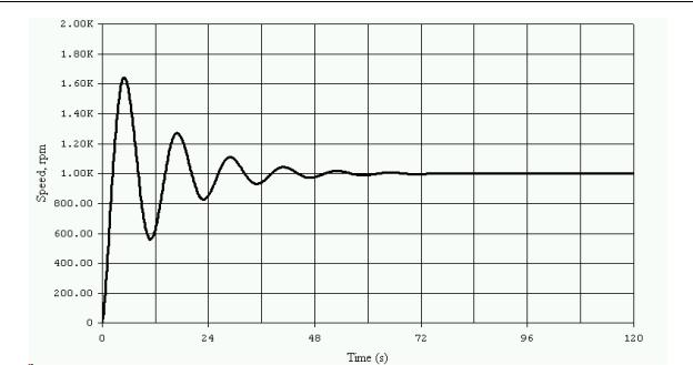
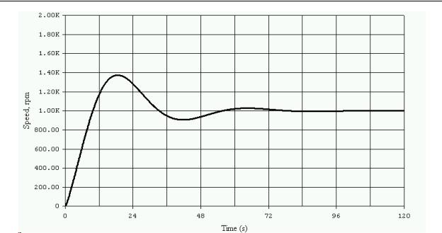
When these PID constants are loaded into the controller and the system is tested with a zero to 1000 rpm step setpoint input, it responds as shown in Figure 10-25.
10-27
Chapter 10 - Closed Loop and PID Control
Figure 10-25 - ZN Tuning Result Using the Open Loop Method
Comparing the system step responses shown in Figures 10-22 and 10-25, we can see that although they are somewhat different in the response time and the amount of hunting, both systems are stable and can be further tuned to the desired response. It should be stressed that the Ziegler-Nichols tuning method is not intended to allow the designer to arrive at the final tuning constants, but instead to provide a stable starting point for further fine tuning of the system.
10-28

Chapter 10 - Closed Loop and PID Control
Chapter 10 Review Questions
10-29