


Chapter 10 - Closed Loop and PID Control
10-8. The PID in Programmable Logic Controllers
Although the general PID concepts and the effects of adjusting the kp, ki and kd constants are the same, when using a programmable logic controller to perform a PID control function, there are some minor differences in the way the PID is adjusted. The PID control unit of a PLC performs all the necessary PID calculations on an iterative basis. That is, the PID calculations are not done continuously, but are triggered by a timing function.
When the timing trigger occurs, the PV and SP are sampled once and digitized, and then all of the proportional, integral, and derivative functions are calculated and summed to produce the CV. The PID then pauses waiting for the next trigger.
The exact parallel PID expression is
|
|
t |
d |
|
|
|
CV = k p (SP − PV ) + ki ∫(SP − PV )dt + kd |
(SP − PV ) |
|||
However, |
dt |
||||
|
0 |
|
|||
since the |
|
|
|
|
|
PLC performs discrete integral and derivative calculations based on the sampling time interval )t, the “discrete” PID performed by a PLC is
|
|
t |
∆(SP − PV ) |
||
|
(SP − PV ) + ki ∑(SP − PV )∆t + kd |
||||
|
CV = k p |
|
|
||
I n t h e |
∆t |
||||
|
0 |
|
|||
numerical |
|
|
integral part of the above |
expression, since SP - PV is the error signal, then |
|
∑t |
(SP − PV )∆t is the sum |
of the areas (the error times the time interval) as illustrated |
0 |
|
|
in Figure 10-15, beginning from the time the system is switched on (t=0) until the present
time t. In a similar manner, the numerical derivative ∆(SP − PV ) is the slope of the error
∆t
signal (the rise divided by the run). The numerator term )(SP-PV) is the present error signal minus the error signal measured in the most recent sample.
Additionally, in order to make the PID tuning more methodical (as will be shown), most PLC manufacturers have replaced ki with what is termed the reset time constant, or integral time constant, Ti. The reset time constant Ti is 1/ki or the inverse of the integral gain constant.2 For similar reasons, the derivative gain constant kd has been
2 If no integral action is desired, Ti is set to zero. Mathematically, this is nonsense because if Ti = 0, ki = 4 which would make the integral gain infinite. However, PID systems are especially programmed to recognize Ti = 0 as a special case and
10-17

Chapter 10 - Closed Loop and PID Control
replaced with the derivative time constant Td, where Td = kd. Therefore, when tuning a PLC operated PID controller, the designer will be adjusting the three constants kp, Ti and Td. Using these constants, our mathematical expression becomes
|
1 |
t |
∆(SP − PV ) |
|
|
CV = k p (SP − PV ) + |
∑(SP − PV )∆t + Td |
|
|||
Ti |
∆t |
||||
|
0 |
|
Some controlled systems respond very slowly. For example, consider the case of a massive oven used to cure the paint on freshly painted products. Even when the oven heaters are fully on, the temperature rate of change may be as slow as a fraction of a degree per minute. If the system is responding this slowly, it would be a waste of processor resources to have the PID continually update at millisecond intervals. For this reason, some of the more sophisticated PID controllers allow the designer to adjust the value of the sampling time interval )t. For slower responding systems, this allows the PID function to be set to update less frequently, which reduces the mathematical processing burden on the system.
10-9. Tuning the PID
Tuning a PID controller system is a subjective process that requires the designer to be very familiar with the characteristics of the system to be controlled and the desired response of the system to changes in the setpoint input. The designer must also take into account the changes in the response of the system if the load on the machine changes. For example, if we are tuning the PID for a subway speed controller, we can expect that the system will respond differently depending on whether the subway is empty or fully loaded with passengers. Additional PID tuning problems can occur if the system being controlled has a nonlinear response to CV inputs (for example, using field current control for controlling the speed of a shunt DC motor). If PID tuning problems occur because of system nonlinearity, one possible solution would be to consider using a fuzzy logic controller instead of a PID. Fuzzy logic controllers can be tuned to match the non-linearity of the system being controlled. Another potential problem in PID tuning can occur with systems that have dual mode controls. These are systems that use one method to adjust the system in one direction and a different method to adjust it in the opposite direction. For example, consider a system in which we need the ability to quickly and accurately control the temperature of a liquid in either the positive or negative direction. Heating the liquid is a simple operation that could involve electric heaters. However, since hot liquids cool slowly, we must rapidly remove the heat using a water cooling system. In this case, not only must the controller regulate the amount of heat that is either injected into or extracted
simply switch off the integral calculation altogether.
10-18

Chapter 10 - Closed Loop and PID Control
from the system, but it must also decide which control system to activate to achieve the desired results. This type of controller sometimes requires the use of two PIDs that are alternately switched on depending on whether the PV is above or below the SP.
Any designer who is familiar with the mathematical fundamentals of PID and the effect that each of the adjustments has on the system can eventually tune a PID to be stable and respond correctly (assuming the system can be tuned at all). However, to efficiently and quickly tune a PID, a designer needs the theoretical knowledge of how a PID functions, a thorough familiarity with how the particular machine being tuned responds to
CV inputs, and experience at tuning PIDs.
It seems as though every designer with experience in tuning PIDs has their own personal way of performing the tuning. However, there are two fundamental methods that can be best used by someone who is new to and unfamiliar with PID tuning. As with nearly all PID tuning methods, both of these methods will give “ballpark” results. That is, they will allow the designer to “rough” tune the PID so that the machine will be stable and will function. Then, from this point, the PID parameters may be further adjusted to achieve results that are closer to the desired performance. There is no PID tuning method that will give the exact desired results on the first try (unless the designer is very lucky!).
Theoretically, it is possible to mathematically calculate the PID coefficients and accurately predict the machine’s performance as a result of the PID tuning; however, in order to do this, the transfer function of the machine being controlled must be accurately mathematically modeled. Modeling the transfer function of a large machine requires determining mechanical parameters (such as mass, friction, damping factors, inertia, windage, and spring constants) and electrical parameters (such as inductance, capacitance, resistance and power factor), many of which are extremely difficult, if not impossible to determine. Therefore, most designers forego this step and simply tune the
PID using somewhat of a trial and error method.
10-10. The “Adjust and Observe” Tuning Method
As the name implies, the “adjust and observe” tuning method involves the making of initial adjustments to the PID constants, observing the response of the machine, and then, knowing how each of the functions of the PID performs, making additional adjustments to correct for undesirable properties of the machine’s response. From our previous discussion of PID performance, we know the following characteristics of PID adjustments.
1.Increasing the proportional gain kp will result in a faster response and will reduce (but not eliminate) offset. However, at the same time, increasing proportional gain will also cause overshoot, hunting, and possible oscillation.
10-19
Chapter 10 - Closed Loop and PID Control
2.Increasing the derivative time constant Td will reduce the hunting and overshoot caused by increasing the proportional gain. However, it will not correct for offset.
3.Decreasing the integral time constant Ti (also called the reset rate or reset time constant) will cause the PID to reduce the offset to near zero. Smaller values of Ti will cause the PID to eliminate the offset at a faster rate. Excessively small (nonzero) values of Ti will cause integral oscillation.
The adjustment procedure is as follows.
1.Initialize the PID constants. This is done by disabling the derivative and integral
functions by setting both Td and Ti to zero, and setting kp to an initial value between 1 and 5.
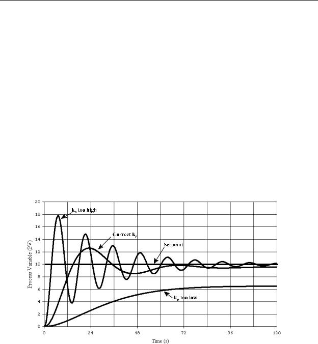
2.With the machine operating, quickly move the setpoint to a new value. Observe the response. Figure 10-17 shows some typical responses with a step setpoint change
from zero to 10 for various values of kp. As shown in the figure, a good preliminary adjustment of kp will result in a response with an overshoot that is approximately
10%-30% of the setpoint change. At this point in the adjustment process we are not concerned about the minor amount of hunting, nor the offset. These problems will be correct later by adjusting Td and Ti respectively.
Figure 10-17 - kp Adjustment Responses
There is usually a large amount of range that kp can have for this adjustment. For example, the three responses shown in Figure 10-17 use kp values of 2, 20, and 200
10-20
Chapter 10 - Closed Loop and PID Control
for this particular system. Although kp = 20 may not be the final value we will use, we will leave it at this value for a starting point.
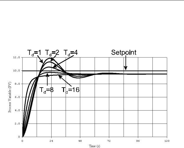
3.Increase Td until the overshoot is reduced to a desired level. If no overshoot is desired, this can also be achieved by further increases in Td. Figure 10-18 shows our example system with kp = 20 and several trial values of Td. For our system, we will attempt to tune the PID to provide minimal overshoot. Therefore, we will use a value of Td = 8.
Figure 10-18 - Td Adjustment
4.Adjust Ti such that the PID will eliminate the offset. Since Ti is the inverse of ki
(Ti = 1/ki), this adjustment should begin with high values of Ti and then be reduced to achieve the desired response. For this adjustment, Ti values that are too large will cause the system to be slow to eliminate the offset, and values of Ti that are too small will cause the PID system to correct the offset too quickly and it will tend to
oscillate. Figure 10-19 shows our example system with kp = 20, Td = 8, and values of 1000, 100, and 10 for Ti. If we are tuning the system for minimal overshoot, a value of Ti = 100 is a good choice.
10-21