


Chapter 10 - Closed Loop and PID Control
Chapter 10 - Closed Loop and PID Control
10-1. Objectives
Upon completion of this chapter, you will know
”the basic parts of a simple closed loop control system.
”why proportional control alone is usually inadequate to maintain a stable system.
”the effect that the addition of derivative control has on a closed loop system.
”the effect that the addition of integral control has on a closed loop system.
”how to tune a PID control system.
10-2. Introduction
One of the greatest strengths of using a programmable machine control, such as a PLC, is in its capability to adapt to changing conditions. When properly designed and programmed, a machine control system is able to sense that a machine is not operating at the desired or optimum conditions and can automatically make adjustments to the machine’s operating parameters so that the desired performance is maintained, even when the surrounding conditions are less than ideal. In this chapter we will discuss various methods of controlling a closed loop system and the advantages and disadvantages of each.
10-3. Simple Closed Loop Systems
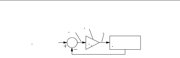
When a control system is designed such that it receives operating information from the machine and makes adjustments to the machine based on this operating information, the system is said to be a closed-loop system, as shown in Figure 10-1. The operating information that the controller receives from the machine is called the process variable (PV) or feedback, and the input from the operator that tells the controller the desired operating point is called the setpoint (SP). When operating, the controller determines whether the machine needs adjustment by comparing (by subtraction) the setpoint and the process variable to produce a difference (the difference is called the error), The error is amplified by a proportional gain1 factor kp in the proportional gain amplifier (sometimes called the error amplifier). The output of the proportional gain amplifier is the control variable (CV) which is connected to the controlling input of the machine. The controller
1In some control systems the term proportional band (with variable P) is used instead of proportional gain. The proportional band is a percentage of the inverse of the proportional gain, or P = 100 / kp .
10-1
Chapter 10 - Closed Loop and PID Control
takes appropriate action to modify the machine’s operating point until the control variable and the setpoint are very nearly equal.
|
PROPORTIONAL GAIN |
|
ERROR |
AMPLIFIER |
|
|
CONTROL VARIABLE (CV) |
|
SETPOINT (SP) |
k p |
CONTROLLED |
MACHINE |
||
PROCESS VARIABLE (PV)
Figure 10-1 - Simple Closed-Loop Control System
It is important to recognize that some closed loop systems do not need to be completely proportional (or analog). They can be partially discrete. For example, the thermostat that controls the heating system in a home is a discrete output device; that is, it provides an output that either switches the heater fully on or completely off. The setpoint for the system is the temperature dial that the homeowner can adjust, and the process variable is the room temperature. If the PV is lower than the SP, the thermostat switches on the CV, in this case a discrete on signal that switches on the heater. The system adapts to external conditions; that is on warm days when the house is comfortable, the thermostat keeps the heater off, and on very cold days, the thermostat operates the heater more often and for longer periods of time. The result is that, despite the changing outdoor temperature, the indoor temperature remains relatively constant.
Some closed loop control systems are totally proportional. Consider, for example, the automobile cruise control. The operator “programs” the system by setting the desired vehicle speed (the SP). The controller then compares this value to the actual speed of the vehicle (the PV), and produces a CV. In this case, the CV results in the accelerator pedal being adjusted so that the vehicle speed is either increased or decreased as needed to maintain a nearly constant speed that is near the SP, even if the auto is climbing or descending hills. The CV signal that controls the accelerator pedal is not discrete, nor would we want it to be. In this application, having a discrete CV signal would result in some very abrupt speed corrections and an uncomfortable ride for the passengers.
When a digital control device (such as a PLC) is used in a control system, the closed loop system may be partially or totally digital. In this case, it still functions as a proportional system, but instead of the signals being voltages or currents, they are digital bytes or words. The error signal is simply the result of digitally subtracting the SP value from the
PV value, which is then multiplied by the proportional gain constant kp. Although the end result can be the same, there are some inherent advantages in using a totally digital system. First, since all numerical processing is done digitally by a microprocessor, the
10-2
Chapter 10 - Closed Loop and PID Control
calibration of the fully digital control system will never drift with temperature or over time. Second, since a microprocessor is present, it is relatively easy to have it perform more sophisticated mathematical functions on the signals such a digital filtering (called digital signal processing, discrete signal processing, or DSP), averaging, numerical integration, and numerical differentiation. As we will see in this chapter, performing advanced mathematical functions on the closed loop signals can vastly improve a system’s response, accuracy and stability. Whenever the closed loop control is performed by a PLC, the actual control calculations are generally performed by a separate coprocessor so that the main processor can be freed to solve the ladder program at high speed. Otherwise, adding closed loop control to a working PLC would drastically slow the PLC scan rate.
10-4. Problems with Simple Closed-Loop Systems
Although the preceding explanation is intended to give the reader an understanding of the fundamentals of closed-loop control systems, unfortunately only a very few types of closed loop systems will work correctly when designed as shown in Figure 10-1. The reason for this is that in order for the machine’s operating point to be near to the value of the SP, the proportional gain kp must be high. However, when a high gain is used, the system becomes unstable and will not adjust its CV correctly. Additionally, if the controlled machine has a delay between the time a CV signal is sent to the machine and the time the machine responds, the control system will tend to overcompensate and over-correct for the error.
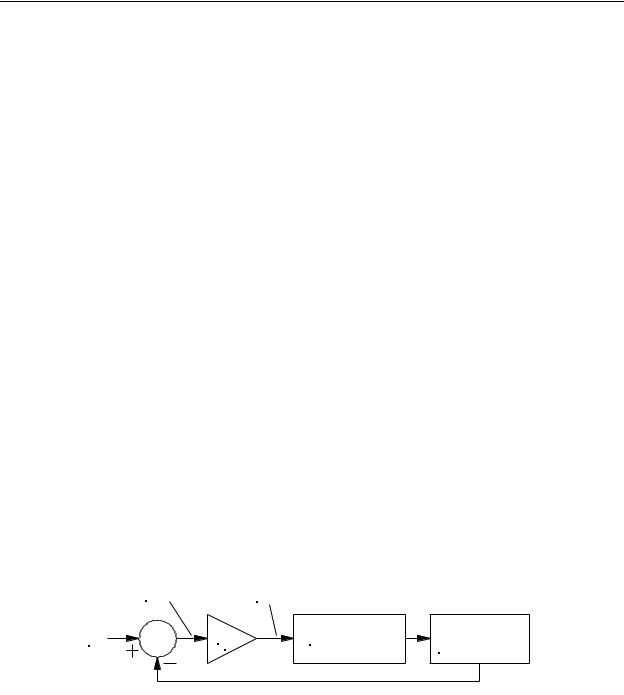
To see why these are potential problems, consider a closed-loop system that controls the speed of a DC motor as shown in Figure 10-2. In this system, the output of the proportional gain amplifier powers the DC motor. The PV for the system is provided by a tacho-generator connected to the motor shaft. The tacho-generator simply outputs a DC voltage proportional to the rotating speed of the shaft. It appears that if we make the SP the same as the tacho-generator’s output (the PV) at the desired speed, the controller will operate the motor at that speed. However, this is not the case.
ERROR |
|
CV |
|
SP |
kp |
DC MOTOR |
TACHO- |
GENERATOR |
PV
Figure 10-2 - Simple Closed-Loop
DC Motor Speed Control System
When the operator inputs a new SP value to change the motor speed, the control system begins automatically adjusting the motor’s speed in an attempt to make the PV
10-3
Chapter 10 - Closed Loop and PID Control
match the SP. However, if the proportional gain amplifier has a low gain kp, the response to the new SP is slow, sluggish, and inaccurate. The reason for this is that as soon as the motor begins accelerating, the tacho-generator begins outputting an increasing voltage as the PV. When this increasing PV voltage is subtracted from the fixed SP, it produces a decreasing error. This means the CV will also decrease which, in turn, will cause the motor speed to increase at a slower rate. This causes the response to be sluggish. Additionally, in our example, let us assume that in order to operate the motor in the desired direction of rotation the CV must be a positive voltage. This means the error must also be some positive voltage. The only way the error voltage can be positive is for the PV voltage to be less than the SP. In other words, the motor speed will “level off” at some value that is less than the SP. It will never reach the desired speed.
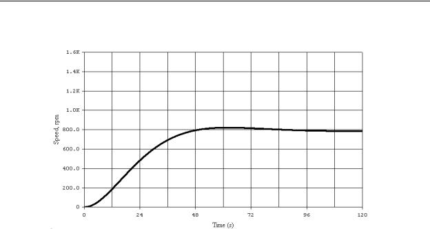
Figure 10-3 is a graph of the speed of a DC motor with respect to time as the motor is accelerated from zero to a SP of 1000 rpm using a closed loop control with low proportional gain. Notice how the motor acceleration is reduced as the motor speed increases which causes the system to take over 90 seconds to settle, and notice that the final motor speed is approximately 350 rpm below the desired setpoint speed of 1000 rpm. This error is called offset.
Figure 10-3 - Motor Speed Control Response
with Low Proportional Gain
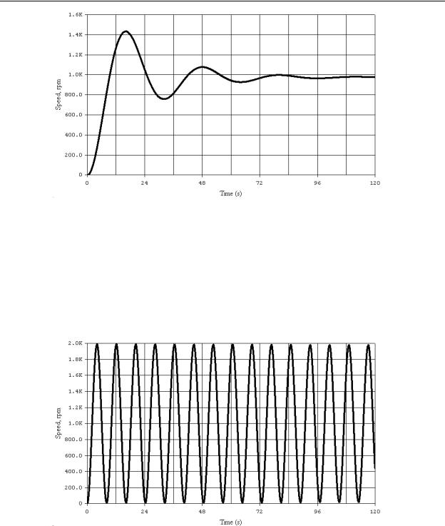
In an attempt to improve both the sluggish response and the offset in our motor speed control, we will now increase the proportional gain kp. Figure 10-4 is a graph of the same system with the proportional gain kp doubled. Notice in this case that the motor speed responds faster and the final speed is closer to the SP than that in Figure 10-3.
10-4
Chapter 10 - Closed Loop and PID Control
However, this system still takes more than a minute to settle and the offset is more than
200rpm below the SP.
Figure 10-4 - Motor Speed Control Response
with Moderate Proportional Gain
Since doubling the proportional gain kp seemed to help the response time and the offset of our system, we will now try a large increase in the proportional gain. Figure 10-5 shows the response of our system with the gain kp increased by a factor of 10. Notice here that the offset is smaller (approximately 25rpm below the SP), however the response now oscillates to both sides of the SP before finally settling. This decaying oscillation is called hunting and in some systems is generally undesirable. It can potentially damage machines with the overstress of mechanical systems and the overspeed of motors. In addition, it is counterproductive because although our motor speed increased rapidly, the system still required nearly two minutes to settle.
10-5
Chapter 10 - Closed Loop and PID Control
Figure 10-5 - Motor Speed Control Response
with High Proportional Gain
If we increase the proportional gain even more, the system becomes unstable. Figure 10-6 shows this condition, which is called oscillation. It is extremely undesirable and, if ignored, will likely be destructive to most closed loop electro mechanical systems.
Any further increase in the proportional gain will cause higher amplitudes of oscillations.
Figure 10-6 - Motor Speed Control Response
with Very High Proportional Gain
10-6