

Chapter 8 - Discrete Position Sensors
8-4. Connecting Discrete Sensors to PLC Inputs
Since discrete PLC inputs can be either sourcing or sinking, it is important to know how to select the sensor output type that will properly interface with the PLC input, and how to wire the PLC input so that it will interface to the sensor correctly. Generally speaking, sensors with sourcing (PNP) outputs should be connected to sinking PLC inputs, and sensors with sinking (NPN) outputs should be connected to sourcing PLC inputs. Connecting sourcing sensor outputs to sourcing PLC inputs, or sinking outputs to sinking inputs, will result in erratic illogical operation at best, or most likely, a system that will not function at all.
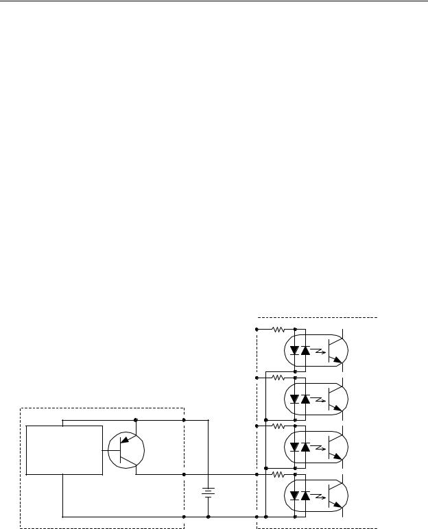
For sourcing (PNP) sensor outputs, the PLC input circuit is wired with the common terminal connected to the common of the sensor as shown in Figure 8-6. When the PNP transistor in the sensor is off, no current flows between the sensor and the PLC, and the
PLC input will be OFF. When the sensor circuitry switches the PNP transistor ON, current flows from the Vcc power supply, through the PNP transistor, through the IN0 opto-isolator in the PLC input, and out of the common terminal to return to the negative side of the power supply. In this case, the PLC input will be ON. For this type of connection, the value of the Vcc voltage must be at least high enough to satisfy the minimum input voltage requirement for the PLC inputs. Notice the simplicity of the connection scheme. The sensor connects directly to the PLC input. No other external signal conditioning circuitry is required.
IN3 
|
IN2 |
|
Vcc |
IN1 |
Programmable |
|
Logic |
|
|
|
|
Proximity |
|
Controller |
|
Discrete |
|
Sensor |
|
Inputs |
Circuitry |
IN0 |
|
Output |
|
|
|
Vcc |
|
Gnd |
COM |
|
Sensor |
|
|
Figure 8-6 - Sourcing Sensor Output Connected to a Sinking PLC Input
8-5
Chapter 8 - Discrete Position Sensors
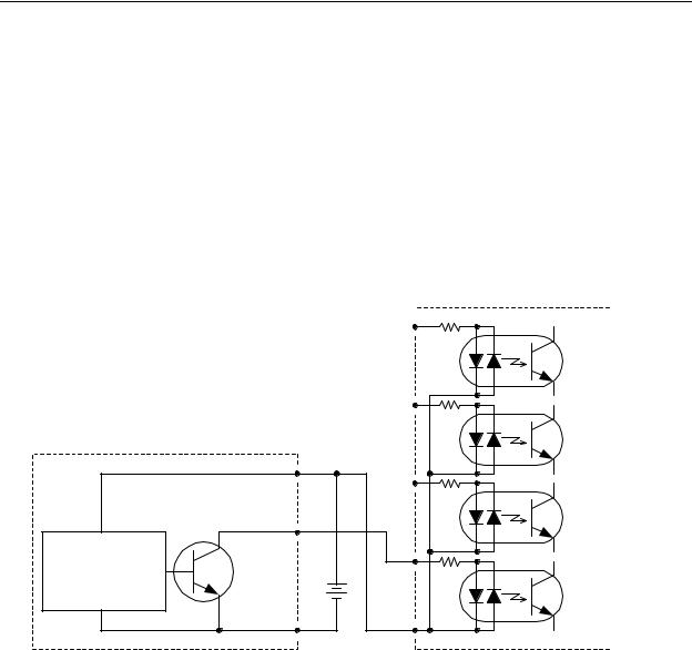
We can also connect a sinking (NPN) sensor output to the same PLC input.
However, since the sensor has a sinking output, the PLC must be rewired as a sourcing input. This can be done by disconnecting the common terminal of the PLC input from the negative side of Vcc and instead connecting it to the positive side of Vcc as shown in Figure 8-7. This connection scheme converts all of the PLC inputs to sourcing; that is, in order to switch the PLC input ON, we must draw current out of the input terminal. In operation, when the NPN transistor in the sensor is OFF, no current flows between the sensor and PLC. However, when the NPN transistor switches ON, current will flow from the positive side of the Vcc supply, into the common terminal of the PLC, up through the opto-isolator, out of the PLC input terminal IN0 and through the NPN transistor to ground. This will switch the PLC input ON. If it is necessary to operate the PLC inputs and the sensor from separate power supplies, it is permissible as long as the negative terminal of both power supplies are connected together.
IN3 
|
IN2 |
|
Vcc |
IN1 |
Programmable |
|
Logic |
|
|
|
|
|
|
Controller |
Output |
|
Discrete |
|
Inputs |
|
Proximity |
IN0 |
|
Sensor |
Vcc |
|
Circuitry |
|
|
Gnd |
COM |
|
Sensor |
|
|
Figure 8-7 - Sinking Sensor Output Connected to a Sourcing PLC Input
8-5. Proximity Sensors
Proximity sensors are discrete sensors that sense when an object has come near to the sensor face. There are four fundamental types of proximity sensors, the inductive proximity sensor, the capacitive proximity sensor, the ultrasonic proximity sensor, and the optical proximity sensor. In order to properly specify and apply proximity sensors, it is important to understand how they operate and to which applications each is best suited.
8-6
Chapter 8 - Discrete Position Sensors
Inductive Proximity Sensors
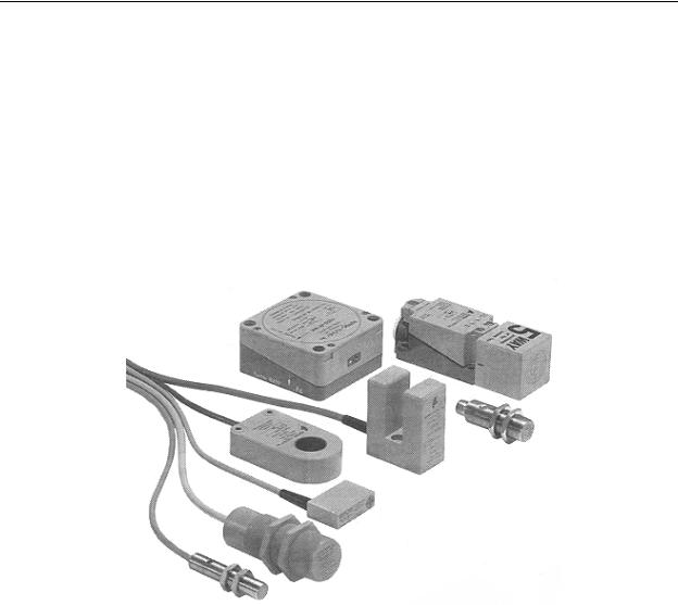
As with all proximity sensors, inductive proximity sensors are available in various sizes and shapes as shown in Figure 8-8. As the name implies, inductive proximity sensors operate on the principle that the inductance of a coil and the power losses in the coil vary as a metallic (or conductive) object is passed near to it. Because of this operating principle, inductive proximity sensors are only used for sensing metal objects. They will not work with non-metallic materials.
Figure 8-8 - Samples of Inductive Proximity Sensors
(Pepperl & Fuchs, Inc.)
To understand how inductive proximity sensors operate, consider the cutaway block diagram shown in Figure 8-9. Mounted just inside the face of the sensor (on the left end) is a coil which is part of the tuned circuit of an oscillator. When the oscillator operates, there is an alternating magnetic field (called a sensing field) produced by the coil. This magnetic field radiates through the face of the sensor (which is non-metallic). The oscillator circuit is tuned such that as long as the sensing field senses non-metallic material (such as air) it will continue to oscillate, it will trigger the trigger circuit, and the output switching device (which inverts the output of the trigger circuit) will be off. The sensor will therefore
8-7
Chapter 8 - Discrete Position Sensors
send an “off” signal through the cable extending from the right side of the sensor in
Figure 8-9.
Figure 8-9 - Inductive Proximity Sensor
Internal Components
(Pepperl & Fuchs, Inc.)
When a metallic object (steel, iron, aluminum, tin, copper, etc.) comes near to the face of the sensor, as shown in Figure 8-10, the alternating magnetic field in the target produces circulating eddy currents inside the material. To the oscillator, these eddy currents are a power loss. As the target moves nearer, the eddy current loss increases which loads the output of oscillator. This loading effect causes the output amplitude of the oscillator to decrease.
Figure 8-10 - Inductive Proximity Sensor
Sensing Target Object
(Pepperl & Fuchs, Inc.)
As long as the oscillator amplitude does not drop below the threshold level of the trigger circuit, the output of the sensor will remain off. However, as shown in Figure 8-11, if the target object moves closer to the face of the sensor, the eddy current loading will cause the oscillator to stall (cease to oscillate). When this happens, the trigger circuit senses the loss of oscillator output and causes the output switching device to switch “on”.
8-8

Chapter 8 - Discrete Position Sensors
Figure 8-11 - Inductive Proximity Sensor
Signals (Pepperl & Fuchs, Inc.)
The sensing range of a proximity sensor is the maximum distance the target object may be from the face of the sensor in order for the sensor to detect it. One parameter affecting the sensing range is the size (diameter) of the sensing coil in the sensor. Small diameter sensors (approximately ¼” in diameter) have typical sensing ranges in the area of 1mm, while large diameter sensors (approximately 3" in diameter) have sensing ranges in the order of 50mm or more. Additionally, since different metals have different values of resistivity (which limits the eddy currents) and permeability (which channels the magnetic field through the target), the type of metal being sensed will affect the sensing range.
Inductive proximity sensor manufacturers derate their sensors based on different metals, with steel being the reference (i.e., having a derating factor of 1.0). Some other approximate derating factors are stainless steel: 0.85, aluminum: 0.40, brass: 0.40, and copper 0.30.
As an example of how to apply the derating factors, assume you are constructing a machine to automatically count copper pennies as they travel down a chute, and the sensing distance will be 5mm. In order to detect copper (derating factor 0.30), you would need to purchase a sensor with a sensing range of 5mm / 0.30 = 16.7mm. Let’s say you found a sensor in stock that has a sensing range of 10mm. If you use this to sense the copper pennies, you would need to mount it near the chute so that the pennies will pass within (10mm)(0.30) = 3mm of the face of the sensor.
Inductive proximity sensors are available in both DC and AC powered models. Most require 3 electrical connections: ground, power, and output. However, there are other variations that require 2 wires and 4 wires. Most sensors are available with a built-in LED that indicates when the sensor is on. One of the first steps a designer should take when using any proximity sensor is to acquire a manufacturer’s catalog and investigate the various types, shapes, and output configurations to determine the best choice for the application.
8-9

Chapter 8 - Discrete Position Sensors
Since the parts of machines are generally constructed of some type of metal, there are an enormous number of possible applications for inductive proximity sensors. They are relatively inexpensive (~$30 and up), extremely reliable, operate from a wide range of power supply voltages, are rugged, and since they are totally self contained, they connect directly to the discrete inputs on a PLC with no additional external components. In many cases, inductive proximity sensors make excellent replacements for mechanical limit switches.
To illustrate some of the wide range of possible applications of inductive proximity sensors (sometimes called inductive prox), consider these uses:
*By placing an inductive prox next to a gear, the prox can sense the passing gear teeth to give rotating speed information. This application is currently used as a speed feedback device in automotive cruise control systems where the prox is mounted in the transmission.
*All helicopters have an inductive prox mounted in the bottom of the rotor gearbox. Should the gears in the gearbox shed any metal chips (indicating an impending catastrophic failure of the gearbox), the inductive prox senses these chips and lights a warning light on the cockpit instrument panel.
*Inductive proxes can be mounted on access doors and panels of machines. The
PLC can be programmed to shut down the machine anytime any of these doors and access panels are opened.
*Very large inductive proxes can be mounted in roadbeds to sense passing automobiles. This technique is currently used to operate traffic lights.
Capacitive Proximity Sensors
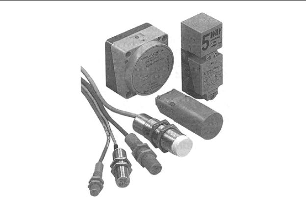
Capacitive proximity sensors are available in shapes and sizes similar to the inductive proximity sensor (as shown in Figure 8-12). However, because of the principle upon which the capacitive proximity sensor operates, applications for the capacitive sensor are somewhat different.
8-10
Chapter 8 - Discrete Position Sensors
Figure 8-12 - Example of Capacitive
Proximity Sensors
(Pepperl & Fuchs, Inc.)
To understand how capacitive proximity sensors operate, consider the cutaway block diagram shown in Figure 8-13. The principle of operation of the sensor is that an internal oscillator will not oscillate until a target material is moved close to the sensor face. The target material varies the capacitance of a capacitor in the face of the sensor that is part of the oscillator circuit. There are two types of capacitive sensor, each with a different way that this sensing capacitor is formed. In the dielectric type of capacitive sensor, there are two side-by-side capacitor plates in the sensor face. For this type of sensor, the external target acts as the dielectric. As the target is moved closer to the sensor face, the change in dielectric increases the capacitance of the internal capacitor, making the oscillator amplitude increase, which in turn causes the sensor to output an “on” signal. The conductive type of sensor operates similarly; however, there is only one capacitor plate in the sensor face. The target becomes the other plate. Therefore, for this type of sensor, it is best if the target is an electrically conductive material (usually metal or water-based).
8-11
Chapter 8 - Discrete Position Sensors
Figure 8-13 - Capacitive Proximity Sensor
Internal Components
(Pepperl & Fuchs, Inc.)
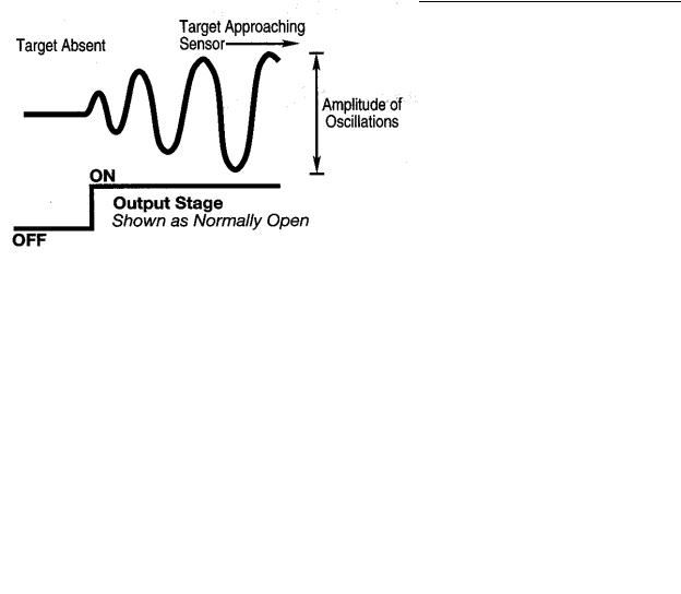
As is shown in the waveform diagram in Figure 8-14, as the target approaches the face of the sensor, the oscillator amplitude increases, which causes the sensor output to switch on.
Figure 8-14 - Capacitive Proximity Sensor
Signals (Pepperl & Fuchs, Inc.)
Dielectric type capacitive proximity sensors will sense both metallic and non-metallic objects. However, in order for the sensor to work properly, it is best if the material being sensed has a high density. Low density materials (foam, bubble wrap, paper, etc.) do not cause a detectable change in the dielectric and consequently will not trigger the sensor.
Conductive type capacitive proximity sensors require that the material being sensed be an electrical conductor. These are ideally suited for sensing metals and conductive liquids. For example, since most disposable liquid containers are made of plastic or cardboard, these sensors have the unique capability to “look” through the container and sense the liquid inside. Therefore, they are ideal for liquid level sensors.
8-12

Chapter 8 - Discrete Position Sensors
Capacitive proximity sensors will sense metal objects just as inductive sensors will.
However, capacitive sensors are much more expensive than the inductive types. Therefore, if the material to be sensed is metal, the inductive sensor is the more economical choice.
Some of the potential applications for capacitive proximity sensors include:
*They can be used as a non-contact liquid level sensor. They can be place outside a container to sense the liquid level inside. This is ideal for milk, juice, or soda bottling operations.
*Capacitive proximity sensors can be used as replacements for pushbuttons and palm switches. They will sense the hand and, since they have no moving parts, they are more reliable than mechanical switches.
*Since they are hermetically sealed, they can be mounted inside liquid tanks to sense the tank fill level.
As with the inductive proximity sensors, capacitive proximity sensors are available with a built-in LED indicator to indicate the output logical state. Also, because capacitive proximity sensors are used to sense materials with a wide range of densities, manufacturers usually provide a sensitivity adjusting screw on the back of the sensor.
Then when the sensor is installed, the sensitivity can be adjusted for best performance in the particular application.
Ultrasonic Proximity Sensors
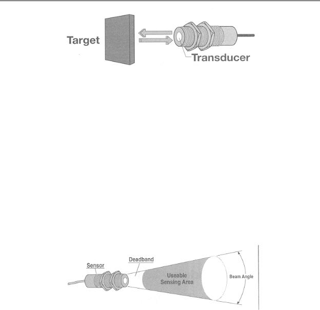
The ultrasonic proximity sensor operates using the same principle as shipboard sonar. As shown in Figure 8-15, an ultrasonic “ping” is sent from the face of the sensor. If a target is located in front of the sensor and is within range, the ping will be reflected by the target and returned to the sensor. When an echo is returned, the sensor detects that a target is present, and by measuring the time delay between the transmitted ping and the returned echo, the sensor can calculate the distance between the sensor and the target.
8-13
Chapter 8 - Discrete Position Sensors
Figure 8-15 - Ultrasonic Proximity Sensor
(Pepperl & Fuchs, Inc.)
As with any proximity sensor, the ultrasonic prox has limitations. The sensor is only capable of sensing a target that is within the sensing range. The sensing range is a funnel shaped area directly in front of the sensor as shown in Figure 8-16. Sound waves travel from the face of the sensor in a cone shaped dispersion pattern bounded by the sensor’s beam angle. However, because the sending and receiving transducers are both located in the face of the sensor, the receiving transducer is “blinded” for a short period of time immediately after the ping is transmitted, similar to the way our eyes are blinded by a flashbulb. This means that any echo that occurs during this “blind” time period will go undetected. These echos will be from targets that are very close to the sensor, within what is called the sensor’s deadband. In addition, because of the finite sensitivity of the receiving transducer, there is a distance beyond which the returning echo cannot be detected. This is the maximum range of the sensor. These constraints define the sensor’s useable sensing area.
Figure 8-16 - Ultrasonic Proximity Sensor
Useable Sensing Area
(Pepperl & Fuchs, Inc.)
Ultrasonic proximity sensors that have a discrete output generally have a switchpoint adjustment provided on the sensor that allows the user to set the target distance at which the sensor output switches on. Note that ultrasonic sensors are also available with analog outputs that will provide an analog signal proportional to the target distance. These types are discussed later in this chapter in the section on distance sensors.
8-14

Chapter 8 - Discrete Position Sensors
Ultrasonic proximity sensors are useful for sensing targets that are beyond the very short operating ranges of inductive and capacitive proximity sensors. Off the shelf ultrasonic proxes are available with sensing ranges of 6 meters or more. They sense dense target materials best such as metals and liquids. They do not work well with soft materials such as cloth, foam rubber, or any material that is a good absorber of sound waves, and they operate poorly with liquids that have surface ripple or waves. Also, for obvious reasons, these sensors will not operate in a vacuum. Since the sound waves must pass through the air, the accuracy of these sensors is subject to the sound propagation time of the air. The most detrimental impact of this is that the sound propagation time of air decreases by 0.17%/degree Celsius. This means that as the air temperature increases, a stationary target will appear to move closer to the sensor. They are not affected by ambient audio noise, nor by wind. However, because of their relatively long useful range, the system designer must take care when using more than one ultrasonic sensor in a system because of the potential for crosstalk between sensors.
One popular use for the ultrasonic proximity sensor is in sensing liquid level. Figure 8-17 shows such an application. Note that since ultrasonic sensors do not perform well with liquids with surface turbulence, a stilling tube is used to reduce the potential turbulence on the surface of the liquid.
8-15