

Radiation Physics for Medical Physiscists - E.B. Podgorsak
.pdf7.3 Compton Scattering (Compton E ect) |
199 |
Fig. 7.8. Fraction of incident photon energy hν transferred in Compton e ect to:
•Maximum energy of recoil electron: (EK)max/(hν); θ = π [see (7.30)]
•Mean energy of recoil electron: EσK/(hν) [see (7.54 below)]
•Maximum energy of scattered photon: hνmax/(hν); θ = 0◦ [see (7.33)]
•Mean energy of the scattered photon: hν /(hν) [see (7.34)]
•Minimum energy of the scattered photon: hνmin/(hν); θ = π [see (7.35)]
Table 7.1, showing that the fractional energy transfer to recoil electrons is quite low at low photon energies (0.02 at hν = 0.01 MeV) and then slowly rises to become 0.44 at hν = 1 MeV and 0.796 at hν = 100 MeV. The mean fraction EσK/(hν) is discussed further in (7.53) and (7.54) below.
Figure 7.8 and Table 7.1 also show the maximum, mean and minimum
fractions (hνmax/hν, hν /hν, hνmin/hν, respectively) of the incident photon energy hν given to the scattered photon. The fractions are calculated as
follows:
hν |
|
hν |
|θ=0 |
|
|
|
|
|
|
|
|
||||||||
|
max |
= |
|
|
|
|
= 1 , |
|
|
|
|
|
|
||||||
|
|
|
|
|
|
|
|
|
|
|
|
|
|
|
|
||||
|
hν |
|
|
hν |
|
|
|
|
|
|
|
|
|
||||||
|
|
|
|
E¯K |
|
|
|
|
|
|
|
|
|
||||||
|
hν |
= 1 − |
, |
|
|
|
|
|
|
|
|
||||||||
|
hν |
hν |
|
|
|
|
|
|
|
|
|
||||||||
hν |
hν |
|θ=π |
1 |
= 1 |
|
(E |
) |
max |
, |
||||||||||
|
min = |
|
|
|
= |
|
− |
|
K |
||||||||||
|
hν |
|
|
|
hν |
|
|
1 + 2ε |
|
|
hν |
|
|||||||
where ε = hν/(mec2).
7.3.4 Di erential Cross Section for Compton Scattering deσcKN/dΩ
(7.33)
(7.34)
(7.35)
The probability or cross section for a Compton interaction between a photon and a “free electron” is given by an expression derived by Oskar Klein and

200 7 Interactions of Photons with Matter
Table 7.1. Fractions of the incident phoyton energy transferred through Compton e ect to the maximum electron kinetic energy (EK)max/(hν); mean electron kinetic energy EσK/(hν); maximum scatterd photon energy hνmax/(hν); mean scattered photon energy hν /(hν); and minimum scattered photon energy hνmin/(hν)
hν (MeV) |
0.01 |
0.1 |
1.0 |
10.0 |
100.0 |
||
(EKσ )max/(hν) |
0.04 |
0.29 |
0.80 |
0.95 |
0.995 |
||
|
Kσ /(hν) |
0.02 |
0.14 |
0.44 |
0.68 |
0.796 |
|
E |
|||||||
hνmax/(hν) |
1.0 |
1.0 |
1.0 |
1.0 |
1.0 |
||
|
/(hν) |
0.98 |
0.86 |
0.56 |
0.32 |
0.21 |
|
hν |
|||||||
hνmin/(hν) |
0.96 |
0.71 |
0.20 |
0.05 |
0.005 |
||
Yoshio Nishina in 1929. The di erential electronic cross section for Compton e ect is given as follows:
deσcKN |
|
re2 |
|
ν |
|
2 |
|
ν |
ν |
− sin2 θ |
|
||||||
|
|
|
|||||||||||||||
|
= |
|
|
|
|
|
+ |
|
|
||||||||
dΩ |
2 |
ν |
|
ν |
ν |
|
|||||||||||
|
= |
re2 |
(1 + cos |
2 |
θ) FKN |
= |
deσTh |
FKN , |
(7.36) |
||||||||
|
|
2 |
|
dΩ |
|||||||||||||
|
|
|
|
|
|
|
|
|
|
|
|
|
|
|
|||
where
deσcKN/dΩ is the di erential Klein-Nishina electronic cross section for the Compton e ect,
νis the frequency of the incident photon,
ν |
is the frequency of the scattered photon, |
θis the scattering angle,
re |
is the classical radius of the electron (2.82 fm), |
FKN |
is the Klein-Nishina form factor, |
deσTh/dΩ is the di erential cross section for Thomson scattering.
The Klein-Nishina form factor FKN for a free electron is given as follows:
F |
|
= |
1 |
|
1 + |
ε2(1 − cos θ)2 |
|
, |
(7.37) |
|
[1 + ε(1 − cos θ)]2 |
[1 + ε(1 − cos θ)](1 + cos2 |
|
||||||
|
KN |
|
|
θ) |
|
||||
where again ε = hν/(mec2).
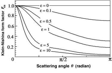
The Klein-Nishina form factor FKN is plotted in Fig. 7.9 against the scattering angle θ for various values of the energy parameter ε. For ε = 0 the form factor is 1 irrespective of the scattering angle θ.
As shown in (7.37) and in Fig. 7.9, the form factor FKN is a complicated function of the scattering angle θ and parameter ε. However, it is easy to show that:
7.3 Compton Scattering (Compton E ect) |
201 |
Fig. 7.9. Atomic form factor for Compton e ect FKN against scattering angle θ
• FKN ≤ 1 for all θ and ε. |
(7.38) |
|
• |
FKN = 1 for θ = 0 at any ε. |
(7.39) |
• |
FKN = 1 for ε = 0 at any θ (Thomson scattering). |
(7.40) |
The di erential electronic cross section for the Compton e ect deσcKN/dΩ when FKN = 1 is equal to the Thomson electronic di erential cross section deσTh/dΩ given in (7.12)
deσcKN |
|
deσTh |
|
re2 |
2 |
|
|
|
|
|FKN=1 = |
|
= |
|
(1 + cos |
|
θ) . |
(7.41) |
dΩ |
dΩ |
2 |
|
|||||
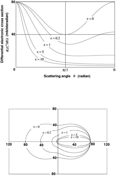
The di erential Compton electronic cross section deσcKN/dΩ is given in Fig. 7.10 against the scattering angle θ for various values of ε ranging from ε ≈ 0 which results in FKN = 1 for all θ, (i.e., Thomson scattering) to ε = 10 for which the FKN causes a significant deviation from the Thomson electronic cross section for all angles θ except for θ = 0.
The data of Fig. 7.10 are replotted in Fig. 7.11 in a polar coordinate system that gives a better illustration of the Compton scattering phenomenon.
•At low ε the probabilities for forward scattering and back scattering are equal and amount to 79.4 mb (Thomson scattering).
•As the energy hν increases the probability for back scattering decreases and the probability for forward scattering remains constant at 79.4 mb.
•The polar diagram of Fig. 7.11 is sometimes colloquially referred to as the “peanut diagram” to help students remember its shape.
At low incident photon energies (Thomson limit) the probabilities for forward scattering and back scattering are equal and twice as large as the probability
202 7 Interactions of Photons with Matter
Fig. 7.10. Di erential electronic cross section for Compton e ect deσcKN/dΩ against scattering angle θ for various values of ε = hν/(mec2), as given by (7.36). The di erential electronic cross section for Compton e ect deσcKN/dΩ for ε = 0 is equal to the di erential electronic cross section for Thomson scattering deσTh/dΩ (see Fig. 7.2)
Fig. 7.11. Polar representation of the angular dependence of the di erential electronic cross section deσcKN/dΩ for Compton scattering, as given by (7.36) and plotted for various values of ε = hν/(mec2). The di erential electronic cross section for Compton e ect deσcKN/dΩ for ε = 0 is equal to the di erential electronic cross section for Thomson scattering deσTh/dΩ (see Fig. 7.3)

7.3 Compton Scattering (Compton E ect) |
203 |
for side scattering. As the incident photon energy, i.e., ε, increases, the scattering becomes increasingly more forward peaked and backscattering rapidly diminishes.
7.3.5 Di erential Energy Transfer Cross Section (deσcKN)tr/dΩ
The di erential energy transfer coe cient (deσcKN)tr/dΩ for the Compton e ect is determined from the di erential electronic cross section deσc/dΩ given in (7.36) as follows:
(d σKN) |
|
d σKN |
|
|
|
|
r2 |
|
|
ν |
|
2 |
|
ν ν |
|
|
|
|
|
ν ν |
|
||||||||||||||
|
E |
|
− |
||||||||||||||||||||||||||||||||
e |
dΩ |
tr |
|
dΩ hν |
|
|
|
|
2 ν |
|
ν ν |
|
|
ν |
|||||||||||||||||||||
c |
= |
e |
c |
|
|
|
K |
= |
|
e |
|
|
|
|
|
|
|
|
|
+ |
|
|
|
sin2 θ |
|
− |
|
||||||||
|
|
|
|
|
|
|
|
|
|
|
|
|
|
|
|
|
|
|
|
|
|
|
|
|
|||||||||||
|
|
|
|
deσTh |
FKN |
|
Kσ |
|
|
re2 |
(1 + cos2 θ) |
|
ε(1 − cos θ) |
|
|
||||||||||||||||||||
|
|
|
= |
E |
= |
|
|
||||||||||||||||||||||||||||
|
|
|
|
hν |
2 |
[1 + ε(1 − cos θ)]3 |
|
||||||||||||||||||||||||||||
|
|
|
|
dΩ |
|
|
|
|
|
|
|
|
|
|
|
|
|
|
|
||||||||||||||||
|
|
|
|
|
|
|
|
|
|
|
|
|
ε2(1 − cos θ)2 |
|
|
|
|
Kσ |
, |
|
|||||||||||||||
|
|
|
|
|
1 + |
|
|
|
|
|
|
|
|
|
E |
(7.42) |
|||||||||||||||||||
|
|
|
|
|
|
|
|
|
|
|
|
|
|
|
|
||||||||||||||||||||
|
|
|
|
|
|
|
|
|
[1 + ε(1 − cos θ)](1 + cos2 θ) hν |
|
|
||||||||||||||||||||||||
where EσK/(hν) is given in Fig. 7.8 and in Table 7.1 for incident photon energies in the range 0.01 MeV ≤ hν ≤ 100 MeV.
7.3.6 Energy Distribution of Recoil Electrons deσcKN/dEK
The di erential electronic Klein-Nishina cross section deσcKN/dEK expressing the initial energy spectrum of Compton recoil electrons averaged over all scattering angles θ is calculated from the general Klein-Nishina relationship for deσcKN/dΩ as follows:
deσcKN(EK) |
deσcKN dΩ dθ |
|
|
|
|
||||||||
|
= |
|
|
|
|
|
|
|
= |
|
|
|
|
|
|
|
|
|
|
|
|
|
|||||
dEK |
dΩ |
|
dθ dEK |
|
|
|
|
||||||
|
|
πre2 |
|
|
|
|
2EK |
|
EK2 |
|
EK2 |
||
= |
|
2 − |
|
+ |
|
+ |
|
||||||
εhν |
ε(hν − EK) |
ε2(hν − EK)2 |
hν(hν − EK) |
||||||||||
where
,
(7.43)
deσcKN/dΩ |
is given in (7.36), |
dΩ/dθ |
is 2π sin θ, |
dθ/dEK |
is (dEK/dθ)−1 with EK(θ) given in (7.29). |
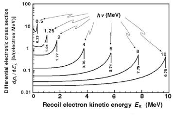
The di erential electronic cross section deσcKN/dEK is plotted in Fig. 7.12 against the kinetic energy EK of the recoil electron for various values of the incident photon energy hν. The following features can now be recognized:
•The distribution of kinetic energies given to the Compton recoil electrons is essentially flat from zero almost up to the maximum electron kinetic energy (EK)max where a higher concentration occurs.
204 7 Interactions of Photons with Matter
Fig. 7.12. Di erential electronic Klein-Nishina cross section per unit kinetic energy deσcKN/dEK calculated from (7.43) and plotted against the kinetic energy of the Compton recoil electron EK for various incident photon energies hν. For a given photon energy the maximum kinetic energy of the recoil electron, calculated from (7.44), is indicated on the graph
• (EK)max is calculated from
(E |
) |
max |
= 2hνε/(1 + 2ε) = hν |
− |
hν |
, |
(7.44) |
|
K |
|
min |
|
|
as given by (7.30). Since, as shown in (7.27), hνmin approaches mec2/2 for high hν, we note that (EK)max approaches hν − (mec2/2).
7.3.7 Total Electronic Klein-Nishina Cross Section for Compton Scattering eσcKN
The total cross section for the Compton scattering on a free electron eσcKN is calculated by integrating the di erential cross section deσcKN/dΩ of (7.36) over the whole solid angle
KN |
= |
deσcKN |
|
|
|
|
|
|
|
|
||||
eσc |
|
|
|
|
dΩ |
|
|
|
|
|
|
|
|
|
|
|
dΩ |
|
|
1 + 2ε |
− |
ε |
+ |
2ε |
− (1 + 2ε)2 . |
||||
|
= 2πre2 |
|
ε2 |
|||||||||||
|
|
|
|
1 + ε 2(1 + ε) |
|
ln(1 + 2ε) |
|
ln(1 + 2ε) |
|
1 + 3ε |
||||
|
|
|
|
|
|
|
|
|
|
|
|
|
(7.45) |
|
The numerical value of eσcKN can also be obtained through a determination of the area under the deσcKN/dθ curve for a given ε. For ε = 0 the area is equal to the Thomson result of 0.665 b [see (7.14)].
Two extreme cases are of special interest, since they simplify the expression for eσcKN:
7.3 Compton Scattering (Compton E ect) |
205 |
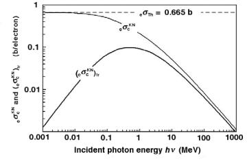
Fig. 7.13. Compton electronic cross section eσcKN and electronic energy transfer cross section (eσcKN)tr for a free electron against incident photon energy hν in the energy range from 0.001 MeV to 1000 MeV, determined from Klein-Nishina Eqs. (7.45) and (7.51), respectively. For very low photon energies eσcKN = eσTh = 0.665 b
• For small incident photon energies hν we get the following relationship:
KN |
= |
8π |
2 |
(1 |
− 2ε + |
26 |
ε |
2 |
− |
133 |
ε |
3 |
+ |
1144 |
ε |
4 |
− . . .) , (7.46) |
||
eσc |
|
re |
|
|
|
|
|
|
|
|
|||||||||
3 |
5 |
|
10 |
|
35 |
|
|||||||||||||
which for ε → 0 approaches the classical Thomson result of (7.14), i.e.,
KN |
ε→0 ≈ eσTh = |
8π |
2 |
= 0.665 b . |
(7.47) |
eσc |
3 |
re |
|||
|
|
|
|
|
|
•For very large incident photon energies hν, i.e., ε 1, we get
KN |
2 1 + 2 ln ε |
|
(7.48) |
||
eσc |
≈ πre |
|
|
. |
|
2ε |
|||||
Figure 7.13 shows the Compton electronic cross section eσcKN as determined by the Klein-Nishina relationship of (7.45) against the incident photon energy hν in the energy range from 0.001 MeV to 1000 MeV. The following features can be identified:
•At low photon energies eσcKN is approximately equal to the classical Thomson cross section eσTh which, with its value of 0.665 b, is independent of photon energy.
•For intermediate photon energies eσcKN decreases gradually with photon energy to read 0.46 b at hν = 0.1 MeV, 0.21 b at hν = 1 MeV, 0.05 b at hν = 10 MeV, and 0.08 b at hν = 100 MeV.
•At very high photon energies hν, the Compton electronic cross section eσcKN attains 1/(hν) dependence, as shown in (7.48).

206 7 Interactions of Photons with Matter
•The Compton electronic cross section eσcKN is independent of atomic number Z of the absorber, since in the Compton theory the electron is assumed free and stationary, i.e., the electron’s binding energy to the atom is assumed to be negligible.
The Compton atomic cross section aσcKN is determined from the electronic cross section of (7.45) using the standard relationship
aσcKN = Z eσcKN , |
(7.49) |
where Z is the atomic number of the absorber.
The Compton mass attenuation coe cient σcKN/ρ is given as follows:
σcKN |
= |
NA |
KN |
= |
ZNA |
KN |
≈ |
1 |
KN |
(7.50) |
||
|
|
|
aσc |
|
|
eσc |
|
NA eσc . |
||||
ρ |
A |
|
A |
2 |
||||||||
The atomic Compton cross section (attenuation coe cient) aσcKN is linearly proportional to Z, while the Compton mass attenuation coe cient σcKN/ρ is essentially independent of Z insofar as Z/A is independent of Z. In reality Z/A ranges from 1 for hydrogen, to 0.5 for low atomic number elements down to 0.4 for high Z, allowing us to make the approximation Z/A ≈ 0.5.
7.3.8 Energy Transfer Cross Section for Compton E ect (eσcKN)tr
The electronic energy transfer cross section (eσcKN)tr is obtained by integrating the di erential energy cross section d(eσcKN)tr/dΩ of (7.42) over all photon scattering angles θ from 0◦ to 180◦ to get
( σKN) |
tr |
= |
|
|
|
|
|
|
|
|
|
|
|
|
|
|
|
|
|
|
||||
e c |
|
|
(1 + 2ε) − |
(1 + 2ε)2 − |
|
|
|
|
|
|
|
|
|
|
|
|||||||||
2 ε2 |
|
|
|
|
|
|
|
|
|
|
||||||||||||||
|
|
|
2(1 + ε)2 |
|
1 + 3ε |
|
|
|
|
|
|
|
|
|
|
|
. |
|||||||
2πre |
|
|
|
|
|
2 |
|
|
|
|
|
|
2 |
|
|
|
|
|
|
|
|
|||
|
|
|
|
|
|
|
|
|
|
|
|
|
|
|
|
|
|
|
|
|
|
|
|
|
|
|
|
|
(1 + ε)(2ε |
|
|
2ε |
|
1) |
|
4ε |
|
|
1 + ε |
1 |
|
1 |
|
|
|||||
|
|
|
|
|
|
|
|
− |
|
− |
|
|
|
|
− |
|
|
|
|
+ |
|
ln(1 + 2ε) |
|
|
|
|
− |
|
ε2(1 + 2ε)2 |
|
|
− 3(1 + 2ε)3 |
ε3 |
− 2ε |
|
2ε3 |
|
|
|||||||||||
|
|
|
|
|
|
|
|
|
|
|
|
|
|
|
|
|
|
|
|
|
|
|
|
|
|
|
|
|
|
|
|
|
|
|
|
|
|
|
|
|
|
|
|
|
|
|
|
|
|
|
|
|
|
|
|
|
|
|
|
|
|
|
|
|
|
|
|
|
|
|
|
|
|
|
(7.51)
In addition to the Compton electronic cross section eσcKN, Fig. 7.13 also shows the energy transfer cross section for the Compton e ect (eσcKN)tr calculated with (7.51) and plotted against the incident photon energy hν in the energy range from 0.001 MeV to 1000 MeV.
Since (eσcKN)tr and eσcKN are related through the following relationship:
(eσcKN)tr = eσcKN |
|
trσ /(hν) , |
(7.52) |
E |
where Eσtr/hν is the mean fraction of the incident photon energy transferred to the kinetic energy of the Compton recoil electron, we can calculate

7.3 Compton Scattering (Compton E ect) |
207 |
EσK/hν as
|
|
Kσ |
(eσcKN)tr |
|
|
|
E |
|
|
||||
|
|
= |
|
, |
(7.53) |
|
|
eσcKN |
|||||
|
hν |
|
|
|||
with (eσcKN)tr and eσcKN given in (7.51) and (7.45), respectively.
Inserting (7.45) and (7.51) into (7.53) gives the following result for the mean fraction of the incident photon energy transferred to the kinetic energy of the recoil electron in Compton e ect EσK/hν:
|
|
Kσ |
= |
|
|
|
|
|
|
|
|
|
|
|
|
|
|
|
|
|
|
|
|
|
|
|
|
|
|
|
E |
|
|
|
|
|
|
|
|
|
|
|
|
|
|
|
|
|
|
|
|
|
|
|
|
|
|
||||
|
|
|
|
|
|
|
|
|
|
|
|
|
|
|
|
|
|
|
|
|
|
|
|
|
|
|
|
|
||
hν |
− |
|
|
− |
|
|
2(1+ε) ln(1+2ε) |
|
ln(1+2ε) |
|
|
|
|
|
|
|
. |
|||||||||||||
|
|
2(1+ε)2 |
|
|
|
|
|
|
|
|
|
|
|
|
|
|||||||||||||||
|
|
|
1+3ε |
|
|
|
(1+ε)(2ε2−2ε−1) |
|
|
4ε2 |
|
! |
1+ε |
|
1 |
|
|
1 |
" |
|
||||||||||
ε2(1+2ε) |
|
|
1+ε |
|
|
ε2(1+2ε)2 |
|
− 3(1+2ε)3 − |
ε3 |
1+3ε |
+ 2ε3 |
|
||||||||||||||||||
|
(1+2ε)2 |
|
|
|
|
|
|
− 2ε |
ln(1 + 2ε) |
|
||||||||||||||||||||
|
|
|
|
|
|
ε2 |
* |
|
− |
|
|
+ + |
|
|
|
− |
|
|
|
|
||||||||||
|
|
|
|
|
|
1+2ε |
|
ε |
2ε |
|
|
(1+2ε)2 |
|
(7.54) |
||||||||||||||||
At first glance (7.54) looks very cumbersome; however, it is simple to use once the appropriate value for ε at a given photon energy hν has been established. For example, an incident photon of energy hν = 1.02 MeV results in ε = 2 that, when inserted into (7.54), gives EσK/(hν) = 0.440
or EσK = 0.440 MeV. The energy of the corresponding scattered photon is hν = hν − EσK = 0.660 MeV.
EσK/(hν) is plotted in Fig. 7.8 (the “Compton Graph”) in the incident photon energy hν range between 0.01 MeV and 100 MeV. Table 7.1 gives several values of EσK/(hν) in the same energy range.
The plot of EσK/(hν) against incident photon energy hν of Fig. 7.8 shows that when low energy photons interact in a Compton process, very little energy is transferred to recoil electrons and most energy goes to the scattered photon. On the other hand, when high energy photons (hν > 10 MeV) interact in a Compton process, most of the incident photon energy is given to the recoil electron and very little is given to the scattered photon.
7.3.9 Binding Energy E ects and Corrections
The Compton electronic cross section eσcKN and energy transfer coe cient (eσcKN)tr were calculated with Klein-Nishina relationships for free electrons and are plotted in Fig. 7.13 with solid curves. At very low incident photon energies the assumption of free electrons breaks down and the electronic binding energy EB a ects the Compton atomic cross sections; the closer is the photon energy hν to EB, the larger is the deviation of the atomic cross section aσc from the calculated free-electron Klein-Nishina cross sections eσcKN.
This discrepancy is evident from Fig. 7.14 that displays, for various absorbers ranging from hydrogen to lead, the atomic cross sections aσc (solid curves) and the calculated Klein-Nishina atomic cross sections aσcKN. Note that aσcKN = Z eσcKN, where eσcKN is calculated with (7.45). It is also shown
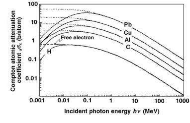
208 7 Interactions of Photons with Matter
Fig. 7.14. Compton atomic cross sections aσc plotted against incident photon energy hν for various absorbers, ranging from hydrogen to lead. The dotted curves represent aσcKN data calculated with Klein-Nishina free-electron relationships; the solid curves represent the aσc data that incorporate the binding e ects of the orbital electrons. The dashed curve represents the Klein-Nishina free electron coe cients eσcKN for the Compton e ect
in Fig. 7.14 that at low incident photon energies hν, the larger is the atomic number Z of the absorber, the more pronounced is the discrepancy and the higher is the energy at which aσc and aσcKN begin to coincide.
Various theories have been developed to account for electronic binding energy e ects on Compton atomic cross sections. Most notable is the method developed by John Hubbell from the National Institute for Science and Technology (NIST) in Washington, USA, who treated the binding energy corrections to the Klein-Nishina relationships in the impulse approximation taking into account all orbital electrons of the absorber atom. This involves applying a multiplicative correction function S(x, Z), referred to as the incoherent scattering function, to the Klein-Nishina atomic cross sections as follows:
daσc |
|
daσcKN |
|
|
|
= |
|
S(x, Z) , |
(7.55) |
dΩ |
|
|||
|
dΩ |
|
||
where x, the momentum transfer variable, stands for sin(θ/2)/λ.
The total Compton atomic cross section aσc is obtained from the following integral:
θ=π |
|
|
aσc = θ=0 |
S(x, Z) deσcKN(θ) , |
(7.56) |