

Теория информации / Cover T.M., Thomas J.A. Elements of Information Theory. 2006., 748p
.pdf15.4 ENCODING OF CORRELATED SOURCES |
555 |
15.4.2Converse for the Slepian–Wolf Theorem
The converse for the Slepian – Wolf theorem follows obviously from the results for a single source, but we will provide it for completeness.
Proof: (Converse to Theorem 15.4.1). As usual, we begin with Fano’s inequality. Let f1, f2, g be fixed. Let I0 = f1(Xn) and J0 = f2(Y n). Then
H (Xn, Y n|I0, J0) ≤ Pe(n)n(log |X| + log |Y|) + 1 = n n, |
(15.178) |
|||||||
where n → 0 as n → ∞. Now adding conditioning, we also have |
|
|||||||
|
|
|
H (Xn|Y n, I0, J0) ≤ n n, |
|
(15.179) |
|||
and |
|
|
|
|
|
|
|
|
|
|
|
H (Y n|Xn, I0, J0) ≤ n n. |
|
(15.180) |
|||
We can write a chain of inequalities |
|
|
|
|
|
|||
|
|
|
(a) |
|
|
|
(15.181) |
|
n(R1 + R2) ≥ H (I0, J0) |
|
|
|
|||||
|
|
|
= I (Xn, Y n; I0, J0) + H (I0, J0|Xn, Y n) |
(15.182) |
||||
|
|
|
(b) |
|
|
|
(15.183) |
|
|
|
|
= I (Xn, Y n; I0, J0) |
|
|
|
||
|
|
|
= H (Xn, Y n) − H (Xn, Y n|I0, J0) |
|
(15.184) |
|||
|
|
|
(c) |
|
|
|
|
|
|
|
|
≥ H (Xn, Y n) − n n |
|
|
|
(15.185) |
|
|
|
|
(d) |
|
|
|
(15.186) |
|
|
|
|
= nH (X, Y ) − n n, |
|
|
|
||
where |
|
|
|
|
|
|
|
|
(a) follows |
from |
the fact that I |
0 { |
1, 2, . . . , 2nR1 |
} |
and J |
0 |
|
|
nR |
} |
|
|
||||
{1, 2, . . . , 2 |
2 |
|
|
|
|
|
||
(b)follows from the fact the I0 is a function of Xn and J0 is a function of Y n
(c)follows from Fano’s inequality (15.178)
(d)follows from the chain rule and the fact that (Xi , Yi ) are i.i.d.
556 NETWORK INFORMATION THEORY
Similarly, using (15.179), we have
(a) |
(15.187) |
nR1 ≥ H (I0) |
|
≥ H (I0|Y n) |
(15.188) |
= I (Xn; I0|Y n) + H (I0|Xn, Y n) |
(15.189) |
(b) |
(15.190) |
= I (Xn; I0|Y n) |
|
= H (Xn|Y n) − H (Xn|I0, J0, Y n) |
(15.191) |
(c) |
|
≥ H (Xn|Y n) − n n |
(15.192) |
(d) |
(15.193) |
= nH (X|Y ) − n n, |
where the reasons are the same as for the equations above. Similarly, we can show that
nR2 ≥ nH (Y |X) − n n. |
(15.194) |
Dividing these inequalities by n and taking the limit as n → ∞, we have
the desired converse. |
|
|
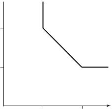
The |
region described in the Slepian – Wolf theorem is illustrated in |
|
Figure |
15.21. |
|
15.4.3Slepian–Wolf Theorem for Many Sources
The results of Section 15.4.2 can easily be generalized to many sources. The proof follows exactly the same lines.
Theorem 15.4.2 Let (X1i , X2i , . . . , Xmi ) be i.i.d. p(x1, x2, . . . , xm). Then the set of rate vectors achievable for distributed source coding with separate encoders and a common decoder is defined by
R(S) > H (X(S)|X(Sc)) |
(15.195) |
for all S {1, 2, . . . , m}, where |
|
R(S) = Ri |
(15.196) |
i S |
|
and X(S) = {Xj : j S}.
15.4 ENCODING OF CORRELATED SOURCES |
557 |
R2 
H(Y )
H(Y |X )
0 |
H(X |Y ) |
H(X ) |
R1 |
|
FIGURE 15.21. Rate region for Slepian – Wolf encoding.
Proof: The proof is identical to the case of two variables and is omitted.
The achievability of Slepian – Wolf encoding has been proved for an i.i.d. correlated source, but the proof can easily be extended to the case of an arbitrary joint source that satisfies the AEP; in particular, it can be extended to the case of any jointly ergodic source [122]. In these cases the entropies in the definition of the rate region are replaced by the corresponding entropy rates.
15.4.4Interpretation of Slepian–Wolf Coding
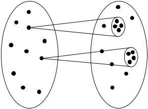
We consider an interpretation of the corner points of the rate region in Slepian – Wolf encoding in terms of graph coloring. Consider the point with rate R1 = H (X), R2 = H (Y |X). Using nH (X) bits, we can encode Xn efficiently, so that the decoder can reconstruct Xn with arbitrarily low probability of error. But how do we code Y n with nH (Y |X) bits? Looking at the picture in terms of typical sets, we see that associated with every Xn is a typical “fan” of Y n sequences that are jointly typical with the given Xn as shown in Figure 15.22.
If the Y encoder knows Xn, the encoder can send the index of the Y n within this typical fan. The decoder, also knowing Xn, can then construct this typical fan and hence reconstruct Y n. But the Y encoder does not know Xn. So instead of trying to determine the typical fan, he randomly
558 NETWORK INFORMATION THEORY
x n |
y n |
FIGURE 15.22. Jointly typical fans.
colors all Y n sequences with 2nR2 colors. If the number of colors is high enough, then with high probability all the colors in a particular fan will be different and the color of the Y n sequence will uniquely define the Y n sequence within the Xn fan. If the rate R2 > H (Y |X), the number of colors is exponentially larger than the number of elements in the fan and we can show that the scheme will have an exponentially small probability of error.
15.5 DUALITY BETWEEN SLEPIAN–WOLF ENCODING AND MULTIPLE-ACCESS CHANNELS
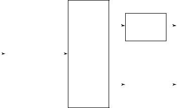
With multiple-access channels, we considered the problem of sending independent messages over a channel with two inputs and only one output. With Slepian – Wolf encoding, we considered the problem of sending a correlated source over a noiseless channel, with a common decoder for recovery of both sources. In this section we explore the duality between the two systems.
In Figure 15.23, two independent messages are to be sent over the channel as X1n and X2n sequences. The receiver estimates the messages from the received sequence. In Figure 15.24 the correlated sources are encoded as “independent” messages i and j . The receiver tries to estimate the source sequences from knowledge of i and j .
In the proof of the achievability of the capacity region for the multipleaccess channel, we used a random map from the set of messages to the


560 NETWORK INFORMATION THEORY
where is the probability the sequences are not typical, Ri are the rates corresponding to the number of codewords that can contribute to the probability of error, and Ii is the corresponding mutual information that corresponds to the probability that the codeword is jointly typical with the received sequence.
In the case of Slepian – Wolf encoding, the corresponding expression
for the probability of error is |
|
|
|
|
|
|
||
Pe(n) ≤ + jointly typical sequences Pr( have the same codeword) |
(15.199) |
|||||||
= + |
nH |
2−nR1 + |
2 |
nH |
2−nR2 + |
nH |
2−n(R1+R2), |
|
2 |
1 terms |
|
2 terms |
2 |
3 terms |
|
|
|
(15.200) where again the probability that the constraints of the AEP are not satisfied is bounded by , and the other terms refer to the various ways in which another pair of sequences could be jointly typical and in the same bin as the given source pair.
The duality of the multiple-access channel and correlated source encoding is now obvious. It is rather surprising that these two systems are duals of each other; one would have expected a duality between the broadcast channel and the multiple-access channel.
15.6BROADCAST CHANNEL
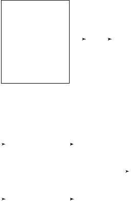
The broadcast channel is a communication channel in which there is one sender and two or more receivers. It is illustrated in Figure 15.25. The basic problem is to find the set of simultaneously achievable rates for communication in a broadcast channel. Before we begin the analysis, let us consider some examples.
Example 15.6.1 (TV station) The simplest example of the broadcast channel is a radio or TV station. But this example is slightly degenerate in the sense that normally the station wants to send the same information to everybody who is tuned in; the capacity is essentially maxp(x) mini I (X; Yi ), which may be less than the capacity of the worst receiver. But we may wish to arrange the information in such a way that the better receivers receive extra information, which produces a better picture or sound, while the worst receivers continue to receive more basic information. As TV stations introduce high-definition TV (HDTV), it may be necessary to encode the information so that bad receivers will receive the
15.6 BROADCAST CHANNEL |
561 |
Y1 |
Decoder |
^ |
|
|
|
W1 |
|
|
|
||
|
|
|
|
X |
|
(W1, W2) |
|
|
Encoder |
|
p(y1, y2|x) |
|
|
||||
|
|
|
|
|
|
Y2 |
Decoder |
^ |
||
|
|
|
W2 |
|
|
|
|
||
|
|
|
|
|
FIGURE 15.25. Broadcast channel.
regular TV signal, while good receivers will receive the extra information for the high-definition signal. The methods to accomplish this will be explained in the discussion of the broadcast channel.
Example 15.6.2 (Lecturer in classroom) A lecturer in a classroom is communicating information to the students in the class. Due to differences among the students, they receive various amounts of information. Some of the students receive most of the information; others receive only a little. In the ideal situation, the lecturer would be able to tailor his or her lecture in such a way that the good students receive more information and the poor students receive at least the minimum amount of information. However, a poorly prepared lecture proceeds at the pace of the weakest student. This situation is another example of a broadcast channel.
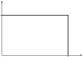
Example 15.6.3 (Orthogonal broadcast channels ) The simplest broadcast channel consists of two independent channels to the two receivers. Here we can send independent information over both channels, and we can achieve rate R1 to receiver 1 and rate R2 to receiver 2 if R1 < C1 and R2 < C2. The capacity region is the rectangle shown in Figure 15.26.
Example 15.6.4 (Spanish and Dutch speaker ) To illustrate the idea of superposition, we will consider a simplified example of a speaker who can speak both Spanish and Dutch. There are two listeners: One understands only Spanish and the other understands only Dutch. Assume for simplicity that the vocabulary of each language is 220 words and that the speaker speaks at the rate of 1 word per second in either language. Then he
562 NETWORK INFORMATION THEORY
R2 |
|
|
C2 |
|
|
0 |
C1 |
R1 |
|
FIGURE 15.26. Capacity region for two orthogonal broadcast channels.
can transmit 20 bits of information per second to receiver 1 by speaking to her all the time; in this case, he sends no information to receiver 2. Similarly, he can send 20 bits per second to receiver 2 without sending any information to receiver 1. Thus, he can achieve any rate pair with R1 + R2 = 20 by simple time-sharing. But can he do better?
Recall that the Dutch listener, even though he does not understand Spanish, can recognize when the word is Spanish. Similarly, the Spanish listener can recognize when Dutch occurs. The speaker can use this to convey information; for example, if the proportion of time he uses each language is 50%, then of a sequence of 100 words, about 50 will be Dutch and about 50 will be Spanish. But there are many ways to order the
100 ≈ 100H ( 1 )
Spanish and Dutch words; in fact, there are about 2 2 ways
50
to order the words. Choosing one of these orderings conveys information to both listeners. This method enables the speaker to send information at a rate of 10 bits per second to the Dutch receiver, 10 bits per second to the Spanish receiver, and 1 bit per second of common information to both receivers, for a total rate of 21 bits per second, which is more than that achievable by simple timesharing. This is an example of superposition of information.
The results of the broadcast channel can also be applied to the case of a single-user channel with an unknown distribution. In this case, the objective is to get at least the minimum information through when the channel is bad and to get some extra information through when the channel is good. We can use the same superposition arguments as in the case of the broadcast channel to find the rates at which we can send information.
15.6 BROADCAST CHANNEL |
563 |
15.6.1Definitions for a Broadcast Channel
Definition A broadcast channel consists of an input alphabet X and two output alphabets, Y1 and Y2, and a probability transition function
p(y1, y2 x). |
|
The |
broadcast channel will be said to be memoryless if |
|||
n |
n| |
n |
) = |
|
n |
|
p(y1 |
, y2 |x |
|
|
i=1 p(y1i , y2i |xi ). |
||
We define |
codes, probability of error, achievability, and capacity regions |
|||||
|
|
|
||||
for the broadcast channel as we did for the multiple-access channel. A ((2nR1 , 2nR2 ), n) code for a broadcast channel with independent information consists of an encoder,
X : ({1, 2, . . . , 2nR1 } × {1, 2, . . . , 2nR2 }) → Xn, |
(15.201) |
and two decoders, |
|
g1 : Y1n → {1, 2, . . . , 2nR1 } |
(15.202) |
and |
|
g2 : Y2n → {1, 2, . . . , 2nR2 }. |
(15.203) |
We define the average probability of error as the probability that the decoded message is not equal to the transmitted message; that is,
Pe(n) = P (g1(Y1n) =W1 or g2(Y2n) =W2), |
(15.204) |
where (W1, W2) are assumed to be uniformly distributed over 2nR1 × 2nR2 .
Definition A rate pair (R1, R2) is said to be achievable for the broad-
cast channel if there exists a sequence of ((2nR1 , 2nR2 ), n) codes with
Pe(n) → 0.
We will now define the rates for the case where we have common information to be sent to both receivers. A ((2nR0 , 2nR1 , 2nR2 ), n) code
for a broadcast channel with common information consists of an encoder,
X : ({1, 2, . . . , 2nR0 } × {1, 2, . . . , 2nR1 } × {1, 2, . . . , 2nR2 }) → Xn,
(15.205)
and two decoders,
g1 : Y1n → {1, 2, . . . , 2nR0 } × {1, 2, . . . , 2nR1 } |
(15.206) |
and |
|
g2 : Y2n → {1, 2, . . . , 2nR0 } × {1, 2, . . . , 2nR2 }. |
(15.207) |
564 NETWORK INFORMATION THEORY
Assuming that the distribution on (W0, W1, W2) is uniform, we can define the probability of error as the probability that the decoded message is not equal to the transmitted message:
Pe(n) = P (g1(Y1n) =(W0, W1) or g2(Zn) =(W0, W2)). |
(15.208) |
Definition A rate triple (R0, R1, R2) is said to be achievable for the
broadcast channel with common information if there exists a sequence of ((2nR0 , 2nR1 , 2nR2 ), n) codes with Pe(n) → 0.
Definition The capacity region of the broadcast channel is the closure of the set of achievable rates.
We observe that an error for receiver Y1n depends only the distribution p(xn, y1n) and not on the joint distribution p(xn, y1n, y2n). Thus, we have the following theorem:
Theorem 15.6.1 The capacity region of a broadcast channel depends only on the conditional marginal distributions p(y1|x) and p(y2|x).
Proof: See the problems. |
|
15.6.2Degraded Broadcast Channels
Definition A broadcast channel is said to be physically degraded if p(y1, y2|x) = p(y1|x)p(y2|y1).
Definition A broadcast channel is said to be stochastically degraded if its conditional marginal distributions are the same as that of a physically degraded broadcast channel; that is, if there exists a distribution p (y2|y1) such that
p(y2|x) = y |
p(y1|x)p (y2|y1). |
(15.209) |
1 |
|
|
Note that since the capacity of a broadcast channel depends only on the conditional marginals, the capacity region of the stochastically degraded broadcast channel is the same as that of the corresponding physically degraded channel. In much of the following, we therefore assume that the channel is physically degraded.