Теория информации / Cover T.M., Thomas J.A. Elements of Information Theory. 2006., 748p

15.6.3Capacity Region for the Degraded Broadcast Channel

We now consider sending independent information over a degraded broadcast channel at rate R1 to Y1 and rate R2 to Y2.

Theorem 15.6.2 The capacity region for sending independent information over the degraded broadcast channel X → Y1 → Y2 is the convex hull of the closure of all (R1, R2) satisfying

for some joint distribution p(u)p(x|u)p(y1, y2|x), where the auxiliary random variable U has cardinality bounded by |U| ≤ min{|X|, |Y1|, |Y2|}.

Proof: (The cardinality bounds for the auxiliary random variable U are derived using standard methods from convex set theory and are not dealt with here.) We first give an outline of the basic idea of superposition coding for the broadcast channel. The auxiliary random variable U will serve as a cloud center that can be distinguished by both receivers Y1 and Y2. Each cloud consists of 2nR1 codewords Xn distinguishable by the receiver Y1. The worst receiver can only see the clouds, while the better receiver can see the individual codewords within the clouds. The formal proof of the achievability of this region uses a random coding argument:

understandable to both Y and Y , while x(i, j ) is the j th satellite codeword in the ith cloud.

Encoding: To send the pair (W1, W2), send the corresponding codeword

Y2) A(n). If there are none such or more than one such, an error is declared.

Y1) A(n). If there are none such or more than one such, an error is declared.

Analysis of the probability of error: By the symmetry of the code generation, the probability of error does not depend on which codeword was

that the third term goes to 0. We can also bound the fourth term in the probability of error as

if n is large enough and R2 < I (U ; Y1) and R1 < I (X; Y1|U ). The above bounds show that we can decode the messages with total probability of error that goes to 0. Hence, there exists a sequence of good ((2nR1 , 2nR2 ), n) codes Cn with probability of error going to 0. With this, we complete the proof of the achievability of the capacity region for the degraded broadcast channel. Gallager’s proof [225] of the converse is outlined in Problem 15.11.

So far we have considered sending independent information to each receiver. But in certain situations, we wish to send common information to both receivers. Let the rate at which we send common information be R0. Then we have the following obvious theorem:

Theorem 15.6.3 If the rate pair (R1, R2) is achievable for a broadcast channel with independent information, the rate triple (R0, R1 − R0, R2 − R0) with a common rate R0 is achievable, provided that R0 ≤ min(R1, R2).

FIGURE 15.28. Physically degraded binary symmetric broadcast channel.

or

α = p2 − p1 . (15.230) 1 − 2p1

We now consider the auxiliary random variable in the definition of the capacity region. In this case, the cardinality of U is binary from the bound of the theorem. By symmetry, we connect U to X by another binary symmetric channel with parameter β, as illustrated in Figure 15.28.

We can now calculate the rates in the capacity region. It is clear by symmetry that the distribution on U that maximizes the rates is the uniform distribution on {0, 1}, so that

Plotting these points as a function of β, we obtain the capacity region in Figure 15.29. When β = 0, we have maximum information transfer to Y2 [i.e., R2 = 1 − H (p2) and R1 = 0]. When β = 12 , we have maximum information transfer to Y1 [i.e., R1 = 1 − H (p1)] and no information transfer to Y2. These values of β give us the corner points of the rate region.

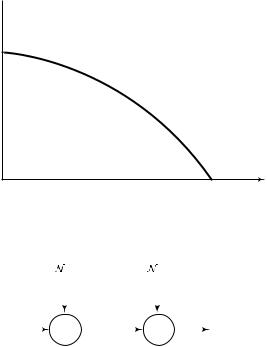
570 NETWORK INFORMATION THEORY

R2

I − H(p2)

FIGURE 15.29. Capacity region of binary symmetric broadcast channel.

cast channel is illustrated in Figure 15.30. We have shown it in the case where one output is a degraded version of the other output. Based on the results of Problem 15.10, it follows that all scalar Gaussian broadcast channels are equivalent to this type of degraded channel.

where Z1 N(0, N1) and Z2 N(0, N2 − N1).

Extending the results of this section to the Gaussian case, we can show

572 NETWORK INFORMATION THEORY

Note that the definition of the encoding functions includes the nonanticipatory condition on the relay. The relay channel input is allowed to depend only on the past observations y11, y12, . . . , y1i−1. The channel is memoryless in the sense that (Yi , Y1i ) depends on the past only through the current transmitted symbols (Xi , X1i ). Thus, for any choice p(w), w W, and code choice X : {1, 2, . . . , 2nR } → Xin and relay functions {fi }ni=1, the joint probability mass function on W × Xn × X1n × Yn × Y1n is given by

n

p(w, x, x1, y, y1) = p(w) p(xi |w)p(x1i |y11, y12, . . . , y1i−1)

denote the conditional probability of error. We define the average probability of error of the code as

The probability of error is calculated under the uniform distribution over the codewords w {1, . . . , 2nR }. The rate R is said to be achievable

by the relay channel if there exists a sequence of (2nR, n) codes with Pe(n) → 0. The capacity C of a relay channel is the supremum of the set

of achievable rates.

We first give an upper bound on the capacity of the relay channel.

Theorem 15.7.1 For any relay channel (X × X1, p(y, y1|x, x1), Y × Y1), the capacity C is bounded above by

Proof: The proof is a direct consequence of a more general max-flow min-cut theorem given in Section 15.10.

This upper bound has a nice max-flow min-cut interpretation. The first term in (15.248) upper bounds the maximum rate of information transfer

from senders X and X1 to receiver Y . The second terms bound the rate from X to Y and Y1.

We now consider a family of relay channels in which the relay receiver is better than the ultimate receiver Y in the sense defined below. Here the max-flow min-cut upper bound in the (15.248) is achieved.

Definition The relay channel (X × X1, p(y, y1|x, x1), Y × Y1) is said to be physically degraded if p(y, y1|x, x1) can be written in the form

Thus, Y is a random degradation of the relay signal Y1.

For the physically degraded relay channel, the capacity is given by the following theorem.

Theorem 15.7.2 The capacity C of a physically degraded relay channel is given by

p(x,x1)

where the supremum is over all joint distributions on X × X1.

Proof:

Converse: The proof follows from Theorem 15.7.1 and by degradedness, since for the degraded relay channel, I (X; Y, Y1|X1) = I (X; Y1|X1).

(3) Slepian – Wolf partitioning, (4) coding for the cooperative multipleaccess channel, (5) superposition coding, and (6) block Markov encoding at the relay and transmitter. We provide only an outline of the proof.

Outline of achievability: We consider B blocks of transmission, each of n symbols. A sequence of B − 1 indices, wi {1, . . . , 2nR }, i = 1, 2, . . . , B − 1, will be sent over the channel in nB transmissions. (Note that as

B → ∞ for a fixed n, the rate R(B − 1)/B is arbitrarily close to R.) We define a doubly indexed set of codewords:

C = {x(w|s), x1(s)} : w {1, 2nR }, s {1, 2nR0 }, x Xn, x1 X1n.

(15.251)

We will also need a partition