Теория информации / Cover T.M., Thomas J.A. Elements of Information Theory. 2006., 748p

≤ 2−1 2 log PU(x) + 2 log PU(x)−1 + 2 log PU(x)−2 + · · ·

(14.100)

where (14.100) is true because there is at most one node at each level that prints out a particular x. More precisely, the nk ’s on the winnowed list for a particular output string x are all different integers. Hence,

simulation of all programs. Then the computer will construct the tree as described above and wait for the particular node p˜ to be assigned. Since the computer executes the same construction as the sender, eventually the node p˜ will be assigned. At this point, the computer will halt and print out the x assigned to that node.

This is an effective (finite, mechanical) procedure for the computer to reconstruct x. However, there is no effective procedure to find the lowest depth node corresponding to x. All that we have proved is that there is

an (infinite) tree with a node corresponding to x at level log 1 + 1.

PU(x)

But this accomplishes our purpose.

With reference to the example, the description of x = 1110 is the path to the node (p3, x3, n3) (i.e., 01), and the description of x = 1111 is the path 00001. If we wish to describe the string 1110, we ask the computer to perform the (simulation) tree construction until node 01 is assigned. Then we ask the computer to execute the program corresponding to node 01 (i.e., p3). The output of this program is the desired string, x = 1110.

The length of the program to reconstruct x is essentially the length of the description of the position of the lowest depth node p˜ corresponding

496 KOLMOGOROV COMPLEXITY

to x in the tree. The length of this program for x is l(p)˜ + c, where

and hence the complexity of x satisfies

14.12KOLMOGOROV SUFFICIENT STATISTIC

Suppose that we are given a sample sequence from a Bernoulli(θ ) process. What are the regularities or deviations from randomness in this sequence? One way to address the question is to find the Kolmogorov complexity K(xn|n), which we discover to be roughly nH0(θ ) + log n + c. Since, for θ =12 , this is much less than n, we conclude that xn has structure and is not randomly drawn Bernoulli( 12 ). But what is the structure? The first attempt to find the structure is to investigate the shortest program p for xn. But the shortest description of p is about as long as p itself; otherwise, we could further compress the description of xn, contradicting the minimality of p . So this attempt is fruitless.

A hint at a good approach comes from an examination of the way in which p describes xn. The program “The sequence has k 1’s; of such sequences, it is the ith” is optimal to first order for Bernoulli(θ ) sequences. We note that it is a two-stage description, and all of the structure of the sequence is captured in the first stage. Moreover, xn is maximally complex given the first stage of the description. The first stage, the description of k, requires log(n + 1) bits and defines a set S = {x {0, 1}n : xi = k}. The second stage requires log |S| = log nk ≈ nH0(xn) ≈ nH0(θ ) bits and reveals nothing extraordinary about xn.

We mimic this process for general sequences by looking for a simple set S that contains xn. We then follow it with a brute-force description of xn in S using log |S| bits. We begin with a definition of the smallest set containing xn that is describable in no more than k bits.

The set S is the smallest set that can be described with no more than k bits and which includes xn. By U(p, n) = S, we mean that running the program p with data n on the universal computer U will print out the indicator function of the set S.

Definition For a given small constant c, let k be the least k such that

Let S be the corresponding set and let p be the program that prints out the indicator function of S . Then we shall say that p is a Kolmogorov minimal sufficient statistic for xn.

All the programs p are “sufficient statistics” in that the complexity of xn given S is maximal. But the minimal sufficient statistic is the shortest “sufficient statistic.”

The equality in the definition above is up to a large constant depending on the computer U . Then k corresponds to the least k for which the twostage description of xn is as good as the best single-stage description of xn. The second stage of the description merely provides the index of xn within the set S ; this takes Kk (xn|n) bits if xn is conditionally maximally complex given the set S . Hence the set S captures all the structure within xn. The remaining description of xn within S is essentially the description of the randomness within the string. Hence S or p is called the Kolmogorov sufficient statistic for xn.

This is parallel to the definition of a sufficient statistic in mathematical statistics. A statistic T is said to be sufficient for a parameter θ if the distribution of the sample given the sufficient statistic is independent of the parameter; that is,

forms a Markov chain in that order. For the Kolmogorov sufficient statistic, the program p is sufficient for the “structure” of the string xn; the remainder of the description of xn is essentially independent of the “structure” of xn. In particular, xn is maximally complex given S .

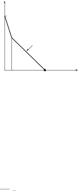
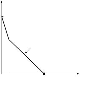
A typical graph of the structure function is illustrated in Figure 14.4. When k = 0, the only set that can be described is the entire set {0, 1}n,

Kk(x)

n

Slope = −1

FIGURE 14.5. Kolmogorov sufficient statistic for a Bernoulli sequence.

sequence among all sequences whose type is in the same bin as k.

Kolmogorov sufficient statistics is k ≈ n log n.

2.Sample from a Markov chain. In the same vein as the preceding

example, consider a sample from a first-order binary Markov chain. In this case again, p will correspond to describing the Markov type of the sequence (the number of occurrences of 00’s, 01’s, 10’s, and 11’s in the sequence); this conveys all the structure in the sequence. The remainder of the description will be the index of the sequence in the set of all sequences of this Markov type. Hence, in this case,

k ≈ 2( 12 log n) = log n, corresponding to describing two elements of the conditional joint type to appropriate accuracy. (The other elements of the conditional joint type can be determined from these two.)

3.Mona Lisa. Consider an image that consists of a gray circle on a white background. The circle is not uniformly gray but Bernoulli with parameter θ . This is illustrated in Figure 14.6. In this case, the best two-stage description is first to describe the size and position of

500 KOLMOGOROV COMPLEXITY

FIGURE 14.6. Mona Lisa.

the circle and its average gray level and then to describe the index of the circle among all the circles with the same gray level. Assuming

an n-pixel image (of size √n by √n), there are about n + 1 possible

gray levels, and there are about (√n)3 distinguishable circles. Hence, k ≈ 52 log n in this case.

14.13MINIMUM DESCRIPTION LENGTH PRINCIPLE

A natural extension of Occam’s razor occurs when we need to describe data drawn from an unknown distribution. Let X1, X2, . . . , Xn be drawn i.i.d. according to probability mass function p(x). We assume that we do not know p(x), but know that p(x) P, a class of probability mass functions. Given the data, we can estimate the probability mass function in P that best fits the data. For simple classes P (e.g., if P has only finitely many distributions), the problem is straightforward, and the maximum likelihood procedure [i.e., find pˆ P that maximizes p(Xˆ 1, X2, . . . , Xn)] works well. However, if the class P is rich enough, there is a problem of overfitting the data. For example, if X1, X2, . . . , Xn are continuous random variables, and if P is the set of all probability distributions, the maximum likelihood estimator given X1, X2, . . . , Xn is a distribution that places a single mass point of weight n1 at each observed value. Clearly, this estimate is too closely tied to actual observed data and does not capture any of the structure of the underlying distribution.

To get around this problem, various methods have been applied. In the simplest case, the data are assumed to come from some parametric distribution (e.g., the normal distribution), and the parameters of the distribution are estimated from the data. To validate this method, the data should be tested to check whether the distribution “looks” normal, and if the data pass the test, we could use this description of the data. A more general procedure is to take the maximum likelihood estimate and smooth it out to obtain a smooth density. With enough data, and appropriate smoothness

SUMMARY 501

conditions, it is possible to make good estimates of the original density. This process is called kernel density estimation.

However, the theory of Kolmogorov complexity (or the Kolmogorov sufficient statistic) suggests a different procedure: Find the p P that minimizes

This is the length of a two-stage description of the data, where we first describe the distribution p and then, given the distribution, construct the

Shannon code and describe the data using log 1 bits. This pro-

p(X1,X2,...,Xn)

cedure is a special case of what is termed the minimum description length (MDL) principle: Given data and a choice of models, choose the model such that the description of the model plus the conditional description of the data is as short as possible.

SUMMARY

Definition. The Kolmogorov complexity K(x) of a string x is

Universality of Kolmogorov complexity. There exists a universal computer U such that for any other computer A,

for any string x, where the constant cA does not depend on x. If U and A are universal, |KU(x) − KA(x)| ≤ c for all x.

502 KOLMOGOROV COMPLEXITY

Kolmogorov complexity and entropy. If X1, X2, . . . are i.i.d. integervalued random variables with entropy H , there exists a constant c such that for all n,

Lower bound on Kolmogorov complexity. There are no more than 2k strings x with complexity K(x) < k. If X1, X2, . . . , Xn are drawn according to a Bernoulli( 12 ) process,

Definition A sequence x is said to be incompressible if

K(x1x2 . . . xn|n)/n → 1.

Strong law of large numbers for incompressible sequences

for every string x {0, 1} , where the constant cA depends only on U and A.

Definition = p: U(p) halts 2−l(p) = Pr(U(p) halts) is the probability that the computer halts when the input p to the computer is a

binary string drawn according to a Bernoulli( 12 ) process.

Properties of

1.is not computable.

2.is a “philosopher’s stone”.

3.is algorithmically random (incompressible).

for all strings x. Thus, the universal probability of a string x is essentially determined by its Kolmogorov complexity.

Let S be the corresponding set and let p be the program that prints out the indicator function of S . Then p is the Kolmogorov minimal sufficient statistic for x.

PROBLEMS

14.1Kolmogorov complexity of two sequences . Let x, y {0, 1} . Argue that K(x, y) ≤ K(x) + K(y) + c.

14.2Complexity of the sum

(a)Argue that K(n) ≤ log n + 2 log log n + c.

(b)Argue that K(n1 + n2) ≤ K(n1) + K(n2) + c.

(c)Give an example in which n1 and n2 are complex but the sum is relatively simple.

14.3Images. Consider an n × n array x of 0’s and 1’s . Thus, x has n2 bits.

504 KOLMOGOROV COMPLEXITY

Find the Kolmogorov complexity K(x | n) (to first order) if:

(a)x is a horizontal line.

(b)x is a square.

(c)x is the union of two lines, each line being vertical or horizontal.

14.4Do computers reduce entropy? Feed a random program P into an universal computer. What is the entropy of the corresponding

output? Specifically, let X = U(P ), where P is a Bernoulli( 12 ) sequence. Here the binary sequence X is either undefined or is in {0, 1} . Let H (X) be the Shannon entropy of X. Argue that H (X) = ∞. Thus, although the computer turns nonsense into sense, the output entropy is still infinite.

14.5Monkeys on a computer . Suppose that a random program is typed into a computer. Give a rough estimate of the probability that the computer prints the following sequence:

(a)0n followed by any arbitrary sequence.

(b)π1π2 . . . πn followed by any arbitrary sequence, where πi is the ith bit in the expansion of π.

(c)0n1 followed by any arbitrary sequence.

(d)ω1ω2 . . . ωn followed by any arbitrary sequence.

(e)A proof of the four-color theorem.

14.6Kolmogorov complexity and ternary programs . Suppose that the

input programs for a universal computer U are sequences in {0, 1, 2} (ternary inputs). Also, suppose that U prints ternary outputs. Let K(x|l(x)) = minU (p,l(x))=x l(p). Show that:

(a)K(xn|n) ≤ n + c.

(b)|xn {0, 1} : K(xn|n) < k| < 3k .

14.7Law of large numbers. Using ternary inputs and outputs as in Problem 14.14.6, outline an argument demonstrating that if a sequence x is algorithmically random [i.e., if K(x|l(x)) ≈ l(x)],

the proportion of 0’s, 1’s, and 2’s in x must each be near 13 . It may be helpful to use Stirling’s approximation n! ≈ (n/e)n.