Добавил:

fench Опубликованный материал нарушает ваши авторские права? Сообщите нам.

Вуз:

Сумский государственный педагогический университет им. Макаренко

Предмет:

Теория вероятностей и математическая статистика

Файл:

Теория информации / Cover T.M., Thomas J.A. Elements of Information Theory. 2006., 748p

.pdf

Скачиваний:

214

Добавлен:

09.08.2013

Размер:

10.58 Mб

Скачать

☆

<<< < Предыдущая 33 34 35 36 37 38 39 40 41 42 43 4445 / 7845 46 47 48 49 50 51 52 53 54 55 56 57 > Следующая >>>

12.4 SPECTRUM ESTIMATION

415

This example shows that the maximum entropy may only be -achiev- able.

12.4SPECTRUM ESTIMATION

Given a stationary zero-mean stochastic process {Xi }, we deﬁne the autocorrelation function as

R(k) = EXi Xi+k .

(12.33)

The Fourier transform of the autocorrelation function for a zero-mean process is the power spectral density S(λ):

S(λ) =	∞
S(λ) =	R(m)e−imλ, −π < λ ≤ π,	(12.34)

m=−∞

√

where i = −1. Since the power spectral density is indicative of the structure of the process, it is useful to form an estimate from a sample of the process.

There are many methods to estimate the power spectrum. The simplest way is to estimate the autocorrelation function by taking sample averages for a sample of length n,

R(k)ˆ =		1		n−k
		1		Xi Xi+k .	(12.35)
	n	−	k	Xi Xi+k .	(12.35)
		−		i=1

If we use all the values of the sample correlation function ˆ · to cal-

R( )

culate the spectrum, the estimate that we obtain from (12.34) does not converge to the true power spectrum for large n. Hence, this method, the periodogram method, is rarely used. One of the reasons for the problem with the periodogram method is that the estimates of the autocorrelation function from the data have different accuracies. The estimates for low values of k (called the lags ) are based on a large number of samples and those for high k on very few samples. So the estimates are more accurate at low k. The method can be modiﬁed so that it depends only on the autocorrelations at low k by setting the higher lag autocorrelations to 0. However, this introduces some artifacts because of the sudden transition to zero autocorrelation. Various windowing schemes have been suggested to smooth out the transition. However, windowing reduces spectral resolution and can give rise to negative power spectral estimates.

In the late 1960s, while working on the problem of spectral estimation for geophysical applications, Burg suggested an alternative method. Instead of

416 MAXIMUM ENTROPY

setting the autocorrelations at high lags to zero, he set them to values that make the fewest assumptions about the data (i.e., values that maximize the entropy rate of the process). This is consistent with the maximum entropy principle as articulated by Jaynes [294]. Burg assumed the process to be stationary and Gaussian and found that the process which maximizes the entropy subject to the correlation constraints is an autoregressive Gaussian process of the appropriate order. In some applications where we can assume an underlying autoregressive model for the data, this method has proved useful in determining the parameters of the model (e.g., linear predictive coding for speech). This method (known as the maximum entropy method or Burg’s method ) is a popular method for estimation of spectral densities. We prove Burg’s theorem in Section 12.6.

12.5ENTROPY RATES OF A GAUSSIAN PROCESS

In Chapter 8 we deﬁned the differential entropy of a continuous random variable. We can now extend the deﬁnition of entropy rates to real-valued stochastic processes.

Deﬁnition The differential entropy rate of a stochastic process {Xi }, Xi R, is deﬁned to be

h(X) = nlim	h(X1, X2, . . . , Xn)	(12.36)
h(X) = nlim	n	(12.36)
→∞

if the limit exists.

Just as in the discrete case, we can show that the limit exists for stationary processes and that the limit is given by the two expressions

h(X) = nlim		h(X1, X2, . . . , Xn)	(12.37)
		n
→∞			(12.38)
= nlim	h(Xn\|Xn−1, . . . , X1).
→∞

For a stationary Gaussian stochastic process, we have

	1
h(X1, X2, . . . , Xn) =	2 log(2π e)n\|K(n)\|,	(12.39)

where the covariance matrix K(n) is Toeplitz with entries R(0), R(1), . . . , R(n − 1) along the top row. Thus, Kij(n) = R(i − j ) = E(Xi − EXi )(Xj

12.6 BURG’S MAXIMUM ENTROPY THEOREM

417

− EXj ). As n → ∞, the density of the eigenvalues of the covariance matrix tends to a limit, which is the spectrum of the stochastic process. Indeed, Kolmogorov showed that the entropy rate of a stationary Gaussian stochastic process can be expressed as

h(	X	)	=	1	log 2π e	+	1	π	log S(λ) dλ.	(12.40)
				2			4π
								−π

The entropy rate is also limn→∞ h(Xn|Xn−1). Since the stochastic process is Gaussian, the conditional distribution is also Gaussian, and hence


the conditional entropy is	1 log 2π eσ 2				, where σ 2	is the variance of the
	2		∞		∞
error in the best estimate of Xn given the inﬁnite past. Thus,
	σ∞2	1		22h(X),		(12.41)
		=
		=	2π e

where h(X) is given by (12.40). Hence, the entropy rate corresponds to the minimum mean-squared error of the best estimator of a sample of the process given the inﬁnite past.

12.6BURG’S MAXIMUM ENTROPY THEOREM

Theorem 12.6.1 The maximum entropy rate stochastic process {Xi } satisfying the constraints

EXi Xi+k = αk ,	k = 0, 1, . . . , p for all i,	(12.42)
is the pth-order Gauss –Markov process of the form
	p
Xi	= − ak Xi−k + Zi ,	(12.43)
	k=1
where the Zi are i.i.d. N(0, σ 2) and a1, a2, . . . , ap , σ 2		are chosen to
satisfy (12.42).

Remark We do not assume that {Xi } is (a) zero mean, (b) Gaussian, or

Proof: Let X1, X2, . . . , Xn be any stochastic process that satisﬁes the constraints (12.42). Let Z1, Z2, . . . , Zn be a Gaussian process with the same covariance matrix as X1, X2, . . . , Xn. Then since the multivariate normal distribution maximizes the entropy over all vector-valued random

418 MAXIMUM ENTROPY

variables under a covariance constraint, we have
h(X1, X2, . . . , Xn) ≤ h(Z1	, Z2, . . . , Zn)	n	(12.44)
= h(Z1	, . . . , Zp ) +	h(Zi \|Zi−1, Zi−2, . . . , Z1)
	i=p+1		(12.45)
		n	(12.45)
		n
≤ h(Z1	, . . . , Zp ) +	h(Zi \|Zi−1, Zi−2, . . . , Zi−p)

i=p+1

(12.46) by the chain rule and the fact that conditioning reduces entropy. Now deﬁne Z1, Z2, . . . , Zn as a pth-order Gauss–Markov process with the same distribution as Z1, Z2, . . . , Zn for all orders up to p. (Existence of such a process will be veriﬁed using the Yule–Walker equations immediately after the proof.) Then since h(Zi |Zi−1, . . . , Zi−p) depends only on

the pth-order distribution, h(Zi |Zi−1, . . . , Zi−p) = h(Zi |Zi−1, . . . , Zi−p), and continuing the chain of inequalities, we obtain

				n
h(X1, X2, . . . , Xn) ≤ h(Z1, . . . , Zp) +				h(Zi \|Zi−1, Zi−2, . . . , Zi−p)
				i=p+1	(12.47)
					(12.47)
= h(Z1, . . . , Zp) +				n
= h(Z1, . . . , Zp) +				h(Zi \|Zi−1, Zi−2, . . . , Zi−p)
				i=p+1	(12.48)
					(12.48)
=	h(Z	, Z	, . . . , Z	),	(12.49)
=	1	2	n

where the last equality follows from the pth-order Markovity of the {Zi }. Dividing by n and taking the limit, we obtain

		1	h(X						lim			1	h(Z	, Z	, . . . , Z			h ,	(12.50)
	lim	1		, X	, . . . , X		)	≤				1				)	=
	lim	n		, X	, . . . , X		)					n				)
		n	1	2		n						n	1	2	n
where
						h =				1	log 2π eσ 2,								(12.51)

										2

which is the entropy rate of the Gauss–Markov process. Hence, the max-

imum entropy rate stochastic process satisfying the constraints	is the
pth-order Gauss–Markov process satisfying the constraints.

A bare-bones summary of the proof is that the entropy of a ﬁnite segment of a stochastic process is bounded above by the entropy of a

12.6 BURG’S MAXIMUM ENTROPY THEOREM

419

segment of a Gaussian random process with the same covariance structure. This entropy is in turn bounded above by the entropy of the minimal order Gauss–Markov process satisfying the given covariance constraints. Such a process exists and has a convenient characterization by means of the Yule–Walker equations given below.

Note on the choice of a1, . . . , ap and σ 2: Given a sequence of covariances R(0), R(1), . . . , R(p), does there exist a pth-order Gauss–Markov process with these covariances? Given a process of the form (12.43), can we choose the ak ’s to satisfy the constraints? Multiplying (12.43) by Xi−l and taking expectations, noting that R(k) = R(−k), we get

p
R(0) = − ak R(−k) + σ 2	(12.52)

and

k=1

R(l) = − ak R(l − k), l = 1, 2, . . . .	(12.53)
k=1

These equations are called the Yule–Walker equations. There are p + 1 equations in the p + 1 unknowns a1, a2, . . . , ap , σ 2. Therefore, we can solve for the parameters of the process from the covariances.

Fast algorithms such as the Levinson algorithm and the Durbin algorithm [433] have been devised to use the special structure of these equations to calculate the coefﬁcients a1, a2, . . . , ap efﬁciently from the covariances. (We set a0 = 1 for a consistent notation.) Not only do the Yule–Walker equations provide a convenient set of linear equations for calculating the ak ’s and σ 2 from the R(k)’s, they also indicate how the autocorrelations behave for lags greater than p. The autocorrelations for high lags are an extension of the values for lags less than p. These values are called the Yule–Walker extension of the autocorrelations. The spectrum of the maximum entropy process is seen to be

S(λ) =		∞
S(λ) =		R(m)e−imλ					(12.54)
m=−∞			σ 2
=			σ 2			, −π ≤ λ ≤ π.	(12.55)

	1 +		p	ikλ	2
	1 +		k=1 ak e−

This is the maximum entropy spectral density subject to the constraints

R(0), R(1), . . . , R(p).

However, for the pth-order Gauss–Markov process, it is possible to calculate the entropy rate directly without calculating the ai ’s. Let Kp be

420 MAXIMUM ENTROPY

the autocorrelation matrix corresponding to this process—the matrix with R0, R1, . . . , Rp along the top row. For this process, the entropy rate is equal to

h = h(Xp |Xp−1, . . . , X0) = h(X0, . . . , Xp ) − h(X0, . . . , Xp−1)

					(12.56)
=	1	log(2π e)p+1\|Kp \| −			1	log(2π e)p\|Kp−1\|

	2				2
					(12.57)
=	1	log(2π e)	\|Kp \|	.	(12.58)
	2	log(2π e)	\|Kp−1\|	.	(12.58)
	2		\|Kp−1\|

In a practical problem, we are generally given a sample sequence X1, X2, . . . , Xn, from which we calculate the autocorrelations. An important question is: How many autocorrelation lags should we consider (i.e., what is the optimum value of p)? A logically sound method is to choose the value of p that minimizes the total description length in a two-stage description of the data. This method has been proposed by Rissanen [442, 447] and Barron [33] and is closely related to the idea of Kolmogorov complexity.

SUMMARY

Maximum entropy distribution. Let f be a probability density satis-

fying the constraints
S f (x)ri (x) = αi for 1 ≤ i ≤ m.		(12.59)
m	λi ri (x), x S, and let λ0	, . . . , λm be cho-
Let f (x) = fλ(x) = eλ0+ i=1

sen so that f satisﬁes (12.59). Then f uniquely maximizes h(f ) over all f satisfying these constraints.

Maximum entropy spectral density estimation. The entropy rate of a stochastic process subject to autocorrelation constraints R0, R1, . . . , Rp is maximized by the pth order zero-mean Gauss-Markov process satisfying these constraints. The maximum entropy rate is

	=	2		\|Kp−1	\|
h		1	log(2π e)	\|Kp \|		,	(12.60)
h			log(2π e)			,	(12.60)

PROBLEMS 421

and the maximum entropy spectral density is

S(λ) =		σ 2			.	(12.61)
S(λ) =	1 +	p	ikλ	2	.	(12.61)
	1 +	k=1 ak e−

PROBLEMS

12.1Maximum entropy . Find the maximum entropy density f ,

deﬁned for x ≥ 0, satisfying EX = α1, E ln X = α2. That is, max-

imize − f ln f subject to xf (x) dx = α1,							(ln x)f (x) dx =
α		, where the integral is over 0	≤	x <	∞.	What family of densi-
	2

ties is this?

12.2Min D(P Q) under constraints on P . We wish to ﬁnd the

(parametric form) of the probability mass function P (x), x {1, 2,

. . .} that minimizes the relative entropy D(P Q) over all P such

that	P (x)gi (x) = αi , i = 1, 2, . . . .
(a)	Use Lagrange multipliers to guess that
	P (x) = Q(x)e i∞=1 λi gi (x)+λ0	(12.62)
	achieves this minimum if there exist λi ’s satisfying the αi
	constraints. This generalizes the theorem on maximum en-
	tropy distributions subject to constraints.

(b)Verify that P minimizes D(P Q).

12.3Maximum entropy processes . Find the maximum entropy rate stochastic process {Xi }∞−∞ subject to the constraints:

(a) EXi2 = 1,	i = 1, 2, . . . .
(b) EXi2 = 1,	EXi Xi+1 = 21 , i = 1, 2, . . . .

(c)Find the maximum entropy spectrum for the processes in parts

(a) and (b).

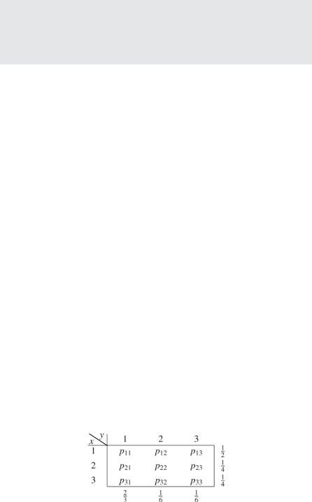
12.4Maximum entropy with marginals. What is the maximum entropy distribution p(x, y) that has the following marginals?

422 MAXIMUM ENTROPY

(Hint: You may wish to guess and verify a more general result.)

12.5Processes with ﬁxed marginals. Consider the set of all densities

with ﬁxed pairwise marginals fX1,X2 (x1, x2), fX2,X3 (x2, x3), . . . , fXn−1,Xn (xn−1, xn). Show that the maximum entropy process with

these marginals is the ﬁrst-order (possibly time-varying) Markov process with these marginals. Identify the maximizing f (x1, x2,

. . . , xn).

12.6Every density is a maximum entropy density . Let f0(x) be a given density. Given r(x), let gα (x) be the density maximizing

h(X) over all f	satisfying		f (x)r(x) dx = α. Now let r(x) =
0	α	= 0								=
ln f (x). Show that g (x)			f (x) for an appropriate choice α
α0. Thus, f0(x) is a maximum entropy density under the constraint
f ln f0 = α0.			n		satisfy EXi Xi+k = Rk , k =
12.7 Mean-squared error . Let			{Xi }i=1		satisfy EXi Xi+k = Rk , k =
0, 1, . . . , p. Consider linear predictors for Xn; that is,
			n−1
	Xˆ n = bi Xn−i .
			i=1
Assume that n > p. Find
	max min E(X				−	ˆ		2	,
	max min E(X			n		X	n	)	,
	f (xn)	b		n			n

where the minimum is over all linear predictors b and the maximum is over all densities f satisfying R0, . . . , Rp .

12.8Maximum entropy characteristic functions . We ask for the max-

imum entropy density f (x), 0 ≤ x ≤ a, satisfying a constraint on the characteristic function (u) = 0a eiux f (x) dx. The answers need be given only in parametric form.

(a)Find the maximum entropy f

=α, at a speciﬁed point u0.

(b)Find the maximum entropy f

satisfying a f (x) cos(u0x) dx

satisfying a f (x) sin(u0x) dx

= β.

(c)Find the maximum entropy density f (x), 0 ≤ x ≤ a, having a

given value of the characteristic function (u0) at a speciﬁed point u0.

(d) What problem is encountered if a = ∞?

PROBLEMS 423

12.9Maximum entropy processes

(a)Find the maximum entropy rate binary stochastic process

{Xi }∞i=−∞, Xi {0, 1}, satisfying Pr{Xi = Xi+1} = 13 for all i.

(b)What is the resulting entropy rate?

12.10Maximum entropy of sums . Let Y = X1 + X2. Find the maxi-

mum entropy density for Y under the constraint EX12 = P1, EX22

= P2:

(a)If X1 and X2 are independent.

(b)If X1 and X2 are allowed to be dependent.

(c)Prove part (a).

12.11Maximum entropy Markov chain. Let {Xi } be a stationary Markov chain with Xi {1, 2, 3}. Let I (Xn; Xn+2) = 0 for all n.

(a)What is the maximum entropy rate process satisfying this

constraint?

(b) What if I (Xn; Xn+2) = α for all n for some given value of

α, 0 ≤ α ≤ log 3?

12.12Entropy bound on prediction error . Let {Xn} be an arbitrary real

= E{Xn+1|X

}. Thus the con-

valued stochastic process. Let Xn+1

is a random variable depending on the n-past

ditional mean X

n+1

. Here Xn+1

is the minimum mean squared error prediction of

Xn+1 given the past.

(a)

Find a

lower bound on the conditional variance E

n+1

{

}} in terms of the conditional differential entropy

− Xn+1) |n

h(Xn+1|X

(b)Is equality achieved when {Xn} is a Gaussian stochastic process?

12.13Maximum entropy rate. What is the maximum entropy rate stochastic process {Xi } over the symbol set {0, 1} for which the probability that 00 occurs in a sequence is zero?

12.14Maximum entropy

(a)What is the parametric-form maximum entropy density f (x) satisfying the two conditions

EX8 = a, EX16 = b?

(b) What is the maximum entropy density satisfying the condition

E(X8 + X16) = a + b?

424 MAXIMUM ENTROPY

12.15Maximum entropy . Find the parametric form of the maximum entropy density f satisfying the Laplace transform condition

f (x)e−x dx = α,

and give the constraints on the parameter.

12.16Maximum entropy processes . Consider the set of all stochastic processes with {Xi }, Xi R, with

R0 = EXi2 = 1, R1 = EXi Xi+1 =	1	.
	2

Find the maximum entropy rate.

12.17Binary maximum entropy . Consider a binary process {Xi }, Xi

{−1, +1}, with R0 = EXi2 = 1 and R1 = EXi Xi+1 = 12 .

(a)Find the maximum entropy process with these constraints.

(b)What is the entropy rate?

(c)Is there a Bernoulli process satisfying these constraints?

12.18Maximum entropy . Maximize h(Z, Vx , Vy , Vz) subject to the en-

ergy constraint E( 12 m V 2 + mgZ) = E0. Show that the resulting distribution yields

E	1	m V 2 =	3	E0	,	EmgZ =	2	E0.
	2		5				5

Thus, 25 of the energy is stored in the potential ﬁeld, regardless of its strength g.

12.19Maximum entropy discrete processes