Теория информации / Cover T.M., Thomas J.A. Elements of Information Theory. 2006., 748p

PROBLEMS 505

14.8Image complexity . Consider two binary subsets A and B (of an n × n grid): for example,

Find general upper and lower bounds, in terms of K(A|n) and

K(B|n), for:

(a)K(Ac|n).

(b)K(A B|n).

(c)K(A ∩ B|n).

14.9Random program. Suppose that a random program (symbols i.i.d. uniform over the symbol set) is fed into the nearest available

computer. To our surprise the first n bits of the binary expansion

√

of 1/ 2 are printed out. Roughly what would you say the proba-

bility is that the next output bit will agree with the corresponding

√

bit in the expansion of 1/ 2 ?

14.10Face–vase illusion

(a)What is an upper bound on the complexity of a pattern on an m × m grid that has mirror-image symmetry about a vertical axis through the center of the grid and consists of horizontal line segments?

(b)What is the complexity K if the image differs in one cell from the pattern described above?

14.11Kolmogorov complexity . Assume that n is very large and known. Let all rectangles be parallel to the frame.

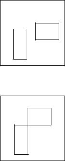
506KOLMOGOROV COMPLEXITY

(a)What is the (maximal) Kolmogorov complexity of the union of two rectangles on an n × n grid?

(b) What if the rectangles intersect at a corner?

(c)What if they have the same (unknown) shape?

(d)What if they have the same (unknown) area?

(e)What is the minimum Kolmogorov complexity of the union of two rectangles? That is, what is the simplest union?

(f)What is the (maximal) Kolmogorov complexity over all images (not necessarily rectangles) on an n × n grid?

14.12Encrypted text . Suppose that English text xn is encrypted into yn by a substitution cypher: a 1-to-1 reassignment of each of the 27 letters of the alphabet (A –Z, including the space character)

to itself. Suppose that the Kolmogorov complexity of the text

xn is K(xn) = n4 . (This is about right for English text. We’re now assuming a 27-symbol programming language, instead of a binary symbol-set for the programming language. So, the length of the shortest program, using a 27-ary programming language, that prints out a particular string of English text of length n, is approximately n/4.)

(a)What is the Kolmogorov complexity of the encryption map?

(b)Estimate the Kolmogorov complexity of the encrypted text yn.

(c)How high must n be before you would expect to be able to decode yn?

14.13Kolmogorov complexity . Consider the Kolmogorov complexity

K(n) over the integers n. If a specific integer n1 has a low Kolmogorov complexity K(n1), by how much can the Kolmogorov complexity K(n1 + k) for the integer n1 + k vary from K(n1)?

14.14Complexity of large numbers. Let A(n) be the set of positive integers x for which a terminating program p of length less than or equal to n bits exists that outputs x. Let B(n) be the complement of A(n) [i.e., B(n) is the set of integers x for which no program of length less than or equal to n outputs x]. Let M(n) be the maximum integer in A(n), and let S(n) be the minimum integer in B(n). What is the Kolmogorov complexity K(M(n)) (approximately)? What is K(S(n)) (approximately)? Which is larger (M(n) or S(n))? Give a reasonable lower bound on M(n) and a reasonable upper bound on S(n).

HISTORICAL NOTES

The original ideas of Kolmogorov complexity were put forth independently and almost simultaneously by Kolmogorov [321, 322], Solomonoff [504], and Chaitin [89]. These ideas were developed further by students of Kolmogorov such as Martin-Lof¨ [374], who defined the notion of algorithmically random sequences and algorithmic tests for randomness, and by Levin and Zvonkin [353], who explored the ideas of universal probability and its relationship to complexity. A series of papers by Chaitin [90] –[92] developed the relationship between algorithmic complexity and mathematical proofs. C. P. Schnorr studied the universal notion of randomness and related it to gambling in [466] –[468].

The concept of the Kolmogorov structure function was defined by Kolmogorov at a talk at the Tallin conference in 1973, but these results were not published. V’yugin pursues this in [549], where he shows that there are some very strange sequences xn that reveal their structure arbitrarily slowly in the sense that Kk (xn|n) = n − k, k < K(xn|n). Zurek [606] – [608] addresses the fundamental questions of Maxwell’s demon and the second law of thermodynamics by establishing the physical consequences of Kolmogorov complexity.

508 KOLMOGOROV COMPLEXITY

Rissanen’s minimum description length (MDL) principle is very close in spirit to the Kolmogorov sufficient statistic. Rissanen [445, 446] finds a low-complexity model that yields a high likelihood of the data. Barron and

Cover [32] argue that the density minimizing K(f ) + log 1 yields

f (Xi )

consistent density estimation.

A nontechnical introduction to the various measures of complexity can be found in a thought-provoking book by Pagels [412]. Additional references to work in the area can be found in a paper by Cover et al. [114] on Kolmogorov’s contributions to information theory and algorithmic complexity. A comprehensive introduction to the field, including applications of the theory to analysis of algorithms and automata, may be found in the book by Li and Vitanyi [354]. Additional coverage may be found in the books by Chaitin [86, 93].

510 NETWORK INFORMATION THEORY

FIGURE 15.1. Multiple-access channel.

FIGURE 15.2. Broadcast channel.

There are other channels, such as the relay channel (where there is one source and one destination, but one or more intermediate sender– receiver pairs that act as relays to facilitate the communication between the source and the destination), the interference channel (two senders and two receivers with crosstalk), and the two-way channel (two sender–receiver pairs sending information to each other). For all these channels, we have only some of the answers to questions about achievable communication rates and the appropriate coding strategies.

All these channels can be considered special cases of a general communication network that consists of m nodes trying to communicate with each other, as shown in Figure 15.3. At each instant of time, the ith node sends a symbol xi that depends on the messages that it wants to send

(X1, Y1)

(Xm, Ym)

(X2, Y2)

FIGURE 15.3. Communication network.

and on past received symbols at the node. The simultaneous transmission of the symbols (x1, x2, . . . , xm) results in random received symbols

(Y1, Y2, . . . , Ym) drawn according to the conditional probability distribution p(y(1), y(2), . . . , y(m)|x(1), x(2), . . . , x(m)). Here p(·|·) expresses the

effects of the noise and interference present in the network. If p(·|·) takes on only the values 0 and 1, the network is deterministic.

Associated with some of the nodes in the network are stochastic data sources, which are to be communicated to some of the other nodes in the network. If the sources are independent, the messages sent by the nodes are also independent. However, for full generality, we must allow the sources to be dependent. How does one take advantage of the dependence to reduce the amount of information transmitted? Given the probability distribution of the sources and the channel transition function, can one transmit these sources over the channel and recover the sources at the destinations with the appropriate distortion?

We consider various special cases of network communication. We consider the problem of source coding when the channels are noiseless and without interference. In such cases, the problem reduces to finding the set of rates associated with each source such that the required sources can be decoded at the destination with a low probability of error (or appropriate distortion). The simplest case for distributed source coding is the Slepian–Wolf source coding problem, where we have two sources that must be encoded separately, but decoded together at a common node. We consider extensions to this theory when only one of the two sources needs to be recovered at the destination.

The theory of flow in networks has satisfying answers in such domains as circuit theory and the flow of water in pipes. For example, for the single-source single-sink network of pipes shown in Figure 15.4, the maximum flow from A to B can be computed easily from the Ford–Fulkerson theorem . Assume that the edges have capacities Ci as shown. Clearly,

512 NETWORK INFORMATION THEORY

C = min{C1 + C2, C2 + C3 + C4, C4 + C5, C1 + C5}

FIGURE 15.4. Network of water pipes.

the maximum flow across any cut set cannot be greater than the sum of the capacities of the cut edges. Thus, minimizing the maximum flow across cut sets yields an upper bound on the capacity of the network. The Ford–Fulkerson theorem [214] shows that this capacity can be achieved.

The theory of information flow in networks does not have the same simple answers as the theory of flow of water in pipes. Although we prove an upper bound on the rate of information flow across any cut set, these bounds are not achievable in general. However, it is gratifying that some problems, such as the relay channel and the cascade channel, admit a simple max-flow min-cut interpretation. Another subtle problem in the search for a general theory is the absence of a source–channel separation theorem, which we touch on briefly in Section 15.10. A complete theory combining distributed source coding and network channel coding is still a distant goal.

In the next section we consider Gaussian examples of some of the basic channels of network information theory. The physically motivated Gaussian channel lends itself to concrete and easily interpreted answers. Later we prove some of the basic results about joint typicality that we use to prove the theorems of multiuser information theory. We then consider various problems in detail: the multiple-access channel, the coding of correlated sources (Slepian–Wolf data compression), the broadcast channel, the relay channel, the coding of a random variable with side information, and the rate distortion problem with side information. We end with an introduction to the general theory of information flow in networks. There are a number of open problems in the area, and there does not yet exist a comprehensive theory of information networks. Even if such a theory is found, it may be too complex for easy implementation. But the theory will be able to tell communication designers how close they are to optimality and perhaps suggest some means of improving the communication rates.

15.1GAUSSIAN MULTIPLE-USER CHANNELS

Gaussian multiple-user channels illustrate some of the important features of network information theory. The intuition gained in Chapter 9 on the Gaussian channel should make this section a useful introduction. Here the key ideas for establishing the capacity regions of the Gaussian multipleaccess, broadcast, relay, and two-way channels will be given without proof. The proofs of the coding theorems for the discrete memoryless counterparts to these theorems are given in later sections of the chapter.

The basic discrete-time additive white Gaussian noise channel with input power P and noise variance N is modeled by

where the Zi are i.i.d. Gaussian random variables with mean 0 and variance N. The signal X = (X1, X2, . . . , Xn) has a power constraint

The Shannon capacity C is obtained by maximizing I (X; Y ) over all random variables X such that EX2 ≤ P and is given (Chapter 9) by

In this chapter we restrict our attention to discrete-time memoryless channels; the results can be extended to continuous-time Gaussian channels.

15.1.1Single-User Gaussian Channel

We first review the single-user Gaussian channel studied in Chapter 9. Here Y = X + Z. Choose a rate R < 12 log(1 + NP ). Fix a good (2nR , n) codebook of power P . Choose an index w in the set 2nR . Send the

wth codeword X(w) from the codebook generated above. The receiver observes Y = X(w) + Z and then finds the index wˆ of the codeword closest to Y. If n is sufficiently large, the probability of error Pr(w =w)ˆ will be arbitrarily small. As can be seen from the definition of joint typicality, this minimum-distance decoding scheme is essentially equivalent to finding the codeword in the codebook that is jointly typical with the received vector Y.

514 NETWORK INFORMATION THEORY

15.1.2Gaussian Multiple-Access Channel with m Users

We consider m transmitters, each with a power P . Let

denote the capacity of a single-user Gaussian channel with signal-to-noise ratio P /N . The achievable rate region for the Gaussian channel takes on the simple form given in the following equations:

Note that when all the rates are the same, the last inequality dominates the others.

Here we need m codebooks, the ith codebook having 2nRi codewords of power P . Transmission is simple. Each of the independent transmitters chooses an arbitrary codeword from its own codebook. The users send these vectors simultaneously. The receiver sees these codewords added together with the Gaussian noise Z.

Optimal decoding consists of looking for the m codewords, one from each codebook, such that the vector sum is closest to Y in Euclidean distance. If (R1, R2, . . . , Rm) is in the capacity region given above, the probability of error goes to 0 as n tends to infinity.