

Теория информации / Cover T.M., Thomas J.A. Elements of Information Theory. 2006., 748p
.pdf15.3 MULTIPLE-ACCESS CHANNEL |
525 |
W1  X1
X1 
|
|
|
^ ^ |
|
p(y | x1, x2) |
|
Y |
|
(W1, W2) |
|
|
|||
W2  Y1
Y1 
FIGURE 15.7. Multiple-access channel.
Definition A ((2nR1 , 2nR2 ), n) code for the multiple-access channel consists of two sets of integers W1 = {1, 2, . . . , 2nR1 } and W2 = {1, 2, . . . ,
2nR2 }, called the message sets, two encoding functions,
X1 : W1 → X1n |
(15.52) |
and |
|
X2 : W2 → X2n, |
(15.53) |
and a decoding function, |
|
g : Yn → W1 × W2. |
(15.54) |
There are two senders and one receiver for this channel. Sender 1 chooses an index W1 uniformly from the set {1, 2, . . . , 2nR1 } and sends the corresponding codeword over the channel. Sender 2 does likewise. Assuming that the distribution of messages over the product set W1 × W2 is uniform (i.e., the messages are independent and equally likely), we define the average probability of error for the ((2nR1 , 2nR2 ), n) code as follows:
Pe(n) = |
1 |
|
Pr |
g(Y n) =(w1 |
, w2)|(w1 |
, w2) sent . |
2n(R1+R2) |
||||||
|
|
(w1,w2) W1×W2 |
|
|
|
|
(15.55)
Definition A rate pair (R1, R2) is said to be achievable for the multiple-
access channel if there exists a sequence of ((2nR1 , 2nR2 ), n) codes with
Pe(n) → 0.

15.3 MULTIPLE-ACCESS CHANNEL |
527 |
X2
Y
X2
FIGURE 15.9. Independent binary symmetric channels.
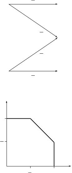
Since the channels are independent, there is no interference between the senders. The capacity region in this case is shown in Figure 15.10.
Example 15.3.2 (Binary multiplier channel ) |
Consider a multiple- |
access channel with binary inputs and output |
|
Y = X1X2. |
(15.59) |
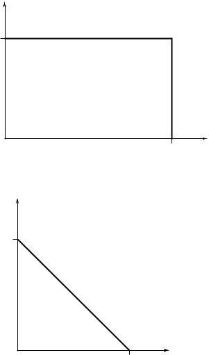
Such a channel is called a binary multiplier channel. It is easy to see that by setting X2 = 1, we can send at a rate of 1 bit per transmission from sender 1 to the receiver. Similarly, setting X1 = 1, we can achieve R2 = 1. Clearly, since the output is binary, the combined rates R1 + R2 of sender 1 and sender 2 cannot be more than 1 bit. By timesharing, we can achieve any combination of rates such that R1 + R2 = 1. Hence the capacity region is as shown in Figure 15.11.
Example 15.3.3 (Binary erasure multiple-access channel ) This multiple-access channel has binary inputs, X1 = X2 = {0, 1}, and a ternary output, Y = X1 + X2. There is no ambiguity in (X1, X2) if Y = 0 or Y = 2 is received; but Y = 1 can result from either (0,1) or (1,0).
528 NETWORK INFORMATION THEORY
R2 |
|
C2 = 1 − H(p2) |
|
0 |
C1 = 1 − H(p1) R1 |
FIGURE 15.10. Capacity region for independent BSCs.
R2 |
|
|
|
C2 = 1 |
|
|
|
0 |
C1 |
= 1 |
R1 |
|
FIGURE 15.11. Capacity region for binary multiplier channel.
We now examine the achievable rates on the axes. Setting X2 = 0, we can send at a rate of 1 bit per transmission from sender 1. Similarly, setting X1 = 0, we can send at a rate R2 = 1. This gives us two extreme points of the capacity region. Can we do better? Let us assume that R1 = 1, so that the codewords of X1 must include all possible binary sequences; X1 would look like a Bernoulli( 12 ) process. This acts like noise for the transmission from X2. For X2, the channel looks like the channel in Figure 15.12. This is the binary erasure channel of Chapter 7. Recalling the results, the
530 NETWORK INFORMATION THEORY
15.3.1 Achievability of the Capacity Region for the Multiple-Access Channel
We now prove the achievability of the rate region in Theorem 15.3.1; the proof of the converse will be left until the next section. The proof of achievability is very similar to the proof for the single-user channel. We therefore only emphasize the points at which the proof differs from the single-user case. We begin by proving the achievability of rate pairs that satisfy (15.58) for some fixed product distribution p(x1)p(x2). In Section 15.3.3 we extend this to prove that all points in the convex hull of (15.58) are achievable.
Proof: |
(Achievability in Theorem |
15.3.1). Fix p(x |
, x ) |
= |
p |
(x )p |
|
(x ). |
||||||||||||||||||
|
nR |
|
|
|
1 |
2 |
|
|
1 |
1 |
|
|
2 |
|
2 |
|||||||||||
|
|
Codebook generation: Generate |
2 |
|
1 |
independent |
codewords |
X1(i), |
||||||||||||||||||
i |
|
1, 2, . . . , 2nR1 |
}, of |
length |
n |
, |
generating |
|
each |
|
element |
|
|
i.i.d. |
||||||||||||
|
{n |
p |
(x |
) |
|
|
nR2 |
|
|
|
codewords X |
|
(j ), |
|||||||||||||
|
i=1 |
|
1 1i |
|
. Similarly, generate 2 |
|
|
independent |
n |
|
|
2 |
2i |
|
|
|
2 |
|
||||||||
j |
|
{ |
|
|
|
|
} |
|
|
|
|
|
|
|
i=1 |
p |
). These |
|||||||||
|
1, 2, . . . , |
2nR2 , generating each element i.i.d. |
|
|
|
|
|
(x |
|
|||||||||||||||||
|
|
|
|
|
|
|
|
|
|
|
|
|
|
|
the senders and the |
|||||||||||
codewords form the codebook, which is revealed to |
|
|
|
|
|
|
|
|
|
|
||||||||||||||||
receiver. |
|
|
|
|
|
|
|
|
|
|
|
|
|
|
|
|
|
|
|
|
|
|
|
|||
|
|
Encoding: To send index i, sender 1 sends the codeword X1(i). Simi- |
||||||||||||||||||||||||
larly, to send j , sender 2 sends X2(j ). |
|
|
|
|
|
|
|
|
|
|
|
|
|
|
|
|||||||||||
|
|
Decoding: Let A(n) denote the set of typical (x1, x2, y) sequences. The |
||||||||||||||||||||||||
|
|
|
|
|
|
|
|
|
|
|
|
|
|
|
|
|
|
|
|
|
|
|
|
|
|
|
receiver Y n chooses the pair (i, j ) such that |
|
|
|
|
|
|
|
|
|
|
|
|
|
|||||||||||||
|
|
|
|
|
|
|
|
(x1(i), x2(j ), y) A(n) |
|
|
|
|
|
|
|
|
(15.60) |
|||||||||
if such a pair (i, j ) exists and is |
unique; otherwise, |
an |
|
error |
is |
de- |
||||||||||||||||||||
clared. |
|
|
|
|
|
|
|
|
|
|
|
|
|
|
|
|
|
|
|
|
|
|
|
|
||
|
|
Analysis of the probability of error: By the symmetry of the random |
||||||||||||||||||||||||
code construction, the conditional probability of error does not depend on which pair of indices is sent. Thus, the conditional probability of error is the same as the unconditional probability of error. So, without loss of generality, we can assume that (i, j ) = (1, 1) was sent.
We have an error if either the correct codewords are not typical with the received sequence or there is a pair of incorrect codewords that are
typical with the received sequence. Define the events |
|
Eij = {(X1(i), X2(j ), Y) A(n)}. |
(15.61) |
532 NETWORK INFORMATION THEORY
on a particular codeword being sent, goes to zero if the conditions of the theorem are met. The above bound shows that the average probability of error, which by symmetry is equal to the probability for an individual codeword, averaged over all choices of codebooks in the random code construction, is arbitrarily small. Hence, there exists at least one code C with arbitrarily small probability of error.
This completes the proof of achievability of the region in (15.58) for a fixed input distribution. Later, in Section 15.3.3, we show that timesharing allows any (R1, R2) in the convex hull to be achieved, completing the proof of the forward part of the theorem.
15.3.2 Comments on the Capacity Region for the Multiple-Access Channel
We have now proved the achievability of the capacity region of the multiple-access channel, which is the closure of the convex hull of the set of points (R1, R2) satisfying
|
|
|
R1 |
< I (X1 |
; Y |X2), |
|
|
(15.73) |
|
|
|
R2 |
< I (X2 |
; Y |X1), |
|
|
(15.74) |
|
|
R1 + R2 |
< I (X1 |
, X2; Y ) |
|
|
(15.75) |
|
for some |
distribution |
|
p1(x1)p2(x2) on X1 × X2. |
For |
a |
particular |
||
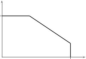
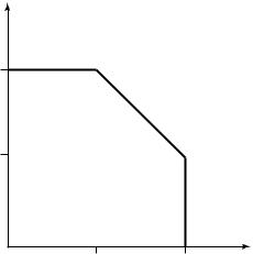
p1(x1)p2(x2), the region is illustrated in Figure 15.14. |
|
|
|
|||||
|
R2 |
|
|
|
|
|
|
|
|
I (X2;Y |X1) |
D |
|
C |
|
|
|
|
|
|
|
|
|
|
|
|
|
|
I (X2;Y ) |
|
|
|
B |
|
|
|
|
|
|
|
|
A |
|
|
|
|
0 |
|
|
I(X1;Y ) |
I(X1;Y |X2) |
R1 |
|
|
|
|
|
|
|
|
|||
FIGURE 15.14. Achievable region of multiple-access channel for a fixed input distribution. |
||||||||
15.3 MULTIPLE-ACCESS CHANNEL |
533 |
Let us now interpret the corner points in the region. Point A corresponds to the maximum rate achievable from sender 1 to the receiver when sender 2 is not sending any information. This is
max R1 = max I (X1; Y |X2). |
(15.76) |
p1(x1)p2(x2)
Now for any distribution p1(x1)p2(x2),
I (X1; Y |X2) = x |
p2(x2)I (X1; Y |X2 = x2) |
(15.77) |
||||||
|
2 |
|
|
|
|
|
|
|
≤ |
max I (X |
|
; |
Y X |
= |
x ), |
(15.78) |
|
x2 |
|
1 |
| 2 |
2 |
||||
since the average is less than the maximum. Therefore, the maximum in (15.76) is attained when we set X2 = x2, where x2 is the value that maximizes the conditional mutual information between X1 and Y . The distribution of X1 is chosen to maximize this mutual information. Thus, X2 must facilitate the transmission of X1 by setting X2 = x2.
The point B corresponds to the maximum rate at which sender 2 can send as long as sender 1 sends at his maximum rate. This is the rate that is obtained if X1 is considered as noise for the channel from X2 to Y . In this case, using the results from single-user channels, X2 can send at a rate I (X2; Y ). The receiver now knows which X2 codeword was used and can “subtract” its effect from the channel. We can consider the channel now to be an indexed set of single-user channels, where the index is the X2 symbol used. The X1 rate achieved in this case is the average mutual information, where the average is over these channels, and each channel occurs as many times as the corresponding X2 symbol appears in the codewords. Hence, the rate achieved is
p(x2)I (X1; Y |X2 = x2) = I (X1; Y |X2). |
(15.79) |
x2
Points C and D correspond to B and A, respectively, with the roles of the senders reversed. The noncorner points can be achieved by time-sharing. Thus, we have given a single-user interpretation and justification for the capacity region of a multiple-access channel.
The idea of considering other signals as part of the noise, decoding one signal, and then “subtracting” it from the received signal is a very useful one. We will come across the same concept again in the capacity calculations for the degraded broadcast channel.
534 NETWORK INFORMATION THEORY
15.3.3 Convexity of the Capacity Region of the Multiple-Access
Channel
We now recast the capacity region of the multiple-access channel in order to take into account the operation of taking the convex hull by introducing a new random variable. We begin by proving that the capacity region is convex.
Theorem 15.3.2 |
The capacity region C of a multiple-access channel |
||||||||||||||||||
is convex [i.e., if (R1, R2) |
C |
|
|
1 |
2 |
|
C |
, then (λR1 |
+ |
(1 |
− |
1 |
|||||||
|
|
and (R |
, R |
) |
|
|
|
λ)R , |
|||||||||||
λR |
2 + |
(1 |
− |
λ)R ) |
C |
for 0 |
≤ |
λ |
≤ |
1]. |
|
|
|
|
|
|
|
|
|
|
|
2 |
|
|
|
|
|
|
|
|
|
|
|
|
|||||
Proof: The idea is time-sharing. Given two sequences of codes at different rates R = (R1, R2) and R = (R1, R2), we can construct a third codebook at a rate λR + (1 − λ)R by using the first codebook for the first λn symbols and using the second codebook for the last (1 − λ)n symbols. The number of X1 codewords in the new code is
nλR1 |
n(1 |
− |
λ)R |
= 2 |
n(λR1 |
+ |
(1 |
− |
λ)R |
) |
, |
(15.80) |
2 |
2 |
1 |
|
|
1 |
|
and hence the rate of the new code is λR + (1 − λ)R . Since the overall probability of error is less than the sum of the probabilities of error for each of the segments, the probability of error of the new code goes to 0 and the rate is achievable.
We can now recast the statement of the capacity region for the multipleaccess channel using a time-sharing random variable Q. Before we prove this result, we need to prove a property of convex sets defined by linear inequalities like those of the capacity region of the multiple-access channel. In particular, we would like to show that the convex hull of two such regions defined by linear constraints is the region defined by the convex combination of the constraints. Initially, the equality of these two sets seems obvious, but on closer examination, there is a subtle difficulty due to the fact that some of the constraints might not be active. This is best illustrated by an example. Consider the following two sets defined by linear inequalities:
C1 = {(x, y) : x ≥ 0, y ≥ 0, x ≤ 10, y ≤ 10, x + y ≤ 100} (15.81)
C2 = {(x, y) : x ≥ 0, y ≥ 0, x ≤ 20, y ≤ 20, x + y ≤ 20}. (15.82)
In this case, the ( 12 , 12 ) convex combination of the constraints defines the region
C = {(x, y) : x ≥ 0, y ≥ 0, x ≤ 15, y ≤ 15, x + y ≤ 60}. (15.83)