Теория информации / Cover T.M., Thomas J.A. Elements of Information Theory. 2006., 748p

14.8 485

every theorem by an effective procedure (Godel’s¨ incompleteness theorem).

The basic idea of the procedure using n bits of is simple: We run all programs until the sum of the masses 2−l(p) contributed by programs that halt equals or exceeds n = 0.ω1ω2 · · · ωn, the truncated version of that we are given. Then, since

we know that the sum of all further contributions of the form 2−l(p) to from programs that halt must also be less than 2−n. This implies that no program of length ≤ n that has not yet halted will ever halt, which enables us to decide the halting or nonhalting of all programs of length ≤ n.

To complete the proof, we must show that it is possible for a computer to run all possible programs in “parallel” in such a way that any program that halts will eventually be found to halt. First, list all possible programs, starting with the null program, :

, 0, 1, 00, 01, 10, 11, 000, 001, 010, 011, . . . . (14.72)

Then let the computer execute one clock cycle of for the first cycle. In the next cycle, let the computer execute two clock cycles of and two clock cycles of the program 0. In the third cycle, let it execute three clock cycles of each of the first three programs, and so on. In this way, the computer will eventually run all possible programs and run them for longer and longer times, so that if any program halts, it will eventually be discovered to halt. The computer keeps track of which program is being executed and the cycle number so that it can produce a list of all the programs that halt. Thus, we will ultimately know whether or not any program of less than n bits will halt. This enables the computer to find any proof of the theorem or a counterexample to the theorem if the theorem can be stated in less than n bits. Knowledge of turns previously unprovable theorems into provable theorems. Here acts as an oracle.

Although seems magical in this respect, there are other numbers that carry the same information. For example, if we take the list of programs and construct a real number in which the ith bit indicates whether program i halts, this number can also be used to decide any finitely refutable question in mathematics. This number is very dilute (in information content) because one needs approximately 2n

486 KOLMOGOROV COMPLEXITY

bits of this indicator function to decide whether or not an n-bit program halts. Given 2n bits, one can tell immediately without any computation whether or not any program of length less than n halts. However, is the most compact representation of this information since it is algorithmically random and incompressible.

What are some of the questions that we can resolve using ? Many of the interesting problems in number theory can be stated as a search for a counterexample. For example, it is straightforward to write a program that searches over the integers x, y, z, and n and halts only if it finds a counterexample to Fermat’s last theorem, which states that

has no solution in integers for n ≥ 3. Another example is Goldbach’s conjecture, which states that any even number is a sum of two primes. Our program would search through all the even numbers starting with 2, check all prime numbers less than it and find a decomposition as a sum of two primes. It will halt if it comes across an even number that does not have such a decomposition. Knowing whether this program halts is equivalent to knowing the truth of Goldbach’s conjecture.

We can also design a program that searches through all proofs and halts only when it finds a proof of the theorem required. This program will eventually halt if the theorem has a finite proof. Hence knowing n bits of , we can find the truth or falsity of all theorems that have a finite proof or are finitely refutable and which can be stated in less than n bits.

3. is algorithmically random.

Theorem 14.8.1 cannot be compressed by more than a constant; that is, there exists a constant c such that

Proof: We know that if we are given n bits of , we can determine whether or not any program of length ≤ n halts. Using K(ω1ω2 · · ·

ωn) bits, we can calculate n bits of , and then we can generate a list of all programs of length ≤ n that halt, together with their corresponding outputs. We find the first string x0 that is not on this list. The string x0 is then the shortest string with Kolmogorov complexity K(x0) > n. The

complexity of this program to print x0 is K( n) + c, which must be at least as long as the shortest program for x0. Consequently,

for all n. Thus, K(ω1ω2 · · · ωn) > n − c, and cannot be compressed by more than a constant.

14.9UNIVERSAL GAMBLING

Suppose that a gambler is asked to gamble sequentially on sequences x {0, 1} . He has no idea of the origin of the sequence. He is given fair odds (2-for-1) on each bit. How should he gamble? If he knew the distribution of the elements of the string, he might use proportional betting because of its optimal growth-rate properties, as shown in Chapter 6. If he believes that the string occurred naturally, it seems intuitive that simpler strings are more likely than complex ones. Hence, if he were to extend the idea of proportional betting, he might bet according to the universal probability of the string. For reference, note that if the gambler knows the string x in advance, he can increase his wealth by a factor of 2l(x) simply by betting all his wealth each time on the next symbol of x. Let the wealth

S(x) associated with betting scheme b(x), b(x) = 1, be given by

Suppose that the gambler bets b(x) = 2−K(x) on a string x. This betting strategy can be called universal gambling. We note that the sum of the bets

b(x) = 2−K(x) ≤ 2−l(p) = ≤ 1, (14.77)

x x p:p halts

and he will not have used all his money. For simplicity, let us assume

that he throws the rest away. For example, the amount of wealth resulting from a bet b(0110) on a sequence x = 0110 is 2l(x)b(x) = 24b(0110) plus

the amount won on all bets b(0110 . . .) on sequences that extend x. Then we have the following theorem:

Theorem 14.9.1 The logarithm of the wealth a gambler achieves on a sequence using universal gambling plus the complexity of the sequence is no smaller than the length of the sequence, or

488 KOLMOGOROV COMPLEXITY

Remark This is the counterpart of the gambling conservation theorem W + H = log m from Chapter 6.

Proof: The proof follows directly from the universal gambling scheme, b(x) = 2−K(x), since

where x x means that x is a prefix of x . Taking logarithms establishes the theorem.

The result can be understood in many ways. For infinite sequences x with finite Kolmogorov complexity,

for all l. Since 2l is the most that can be won in l gambles at fair odds, this scheme does asymptotically as well as the scheme based on knowing the sequence in advance. For example, if x = π1π2 · · · πn · · ·, the digits in the expansion of π , the wealth at time n will be Sn = S(xn) ≥ 2n−c for all n.

If the string is actually generated by a Bernoulli process with parameter p, then

S(X1 . . . Xn) ≥ 2n−nH0(Xn)−2 log n−c ≈ 2n(1−H0(p)−2 logn n − nc ), (14.81)

which is the same to first order as the rate achieved when the gambler knows the distribution in advance, as in Chapter 6.

From the examples we see that the universal gambling scheme on a random sequence does asymptotically as well as a scheme that uses prior knowledge of the true distribution.

14.10OCCAM’S RAZOR

In many areas of scientific research, it is important to choose among various explanations of data observed. After choosing the explanation, we wish to assign a confidence level to the predictions that ensue from the laws that have been deduced. For example, Laplace considered the probability that the sun will rise again tomorrow given that it has risen every day in recorded history. Laplace’s solution was to assume that the rising of the sun was a Bernoulli(θ ) process with unknown parameter θ . He assumed that θ was uniformly distributed on the unit interval. Using

the observed data, he calculated the posterior probability that the sun will rise again tomorrow and found that it was

P (Xn+1 = 1|Xn = 1, Xn−1 = 1, . . . , X1 = 1)

which he put forward as the probability that the sun will rise on day n + 1 given that it has risen on days 1 through n.

Using the ideas of Kolmogorov complexity and universal probability, we can provide an alternative approach to the problem. Under the universal probability, let us calculate the probability of seeing a 1 next after having observed n 1’s in the sequence so far. The conditional probability that the next symbol is a 1 is the ratio of the probability of all sequences with initial segment 1n and next bit equal to 1 to the probability of all sequences with initial segment 1n. The simplest programs carry most of the probability; hence we can approximate the probability that the next bit is a 1 with the probability of the program that says “Print 1’s forever.”

Estimating the probability that the next bit is 0 is more difficult. Since any program that prints 1n0 . . . yields a description of n, its length should at least be K(n), which for most n is about log n + O(log log n), and hence ignoring second-order terms, we have

Hence, the conditional probability of observing a 0 next is

which is similar to the result p(0|1n) = 1/(n + 1) derived by Laplace.

492 KOLMOGOROV COMPLEXITY

string by looking for the corresponding node in the tree. This is the basis for the following tree construction procedure.

To overcome the problem of noncomputability of PU(x), we use a modified approach, trying to construct a code tree directly. Unlike Huffman coding, this approach is not optimal in terms of minimum expected codeword length. However, it is good enough for us to derive a code for which

Before we get into the details of the proof, let us outline our approach. We want to construct a code tree in such a way that strings with high probability have low depth. Since we cannot calculate the probability of a string, we do not know a priori the depth of the string on the tree. Instead, we assign x successively to the nodes of the tree, assigning x to nodes closer and closer to the root as our estimate of PU(x) improves. We want the computer to be able to recreate the tree and use the lowest depth node corresponding to the string x to reconstruct the string.

We now consider the set of programs and their corresponding outputs {(p, x)}. We try to assign these pairs to the tree. But we immediately come across a problem— there are an infinite number of programs for a given string, and we do not have enough nodes of low depth. However, as we shall show, if we trim the list of program-output pairs, we will be able to define a more manageable list that can be assigned to the tree.

Tree construction procedure: For the universal computer U, we simulate all programs using the technique explained in Section 14.8. We list all binary programs:

, 0, 1, 00, 01, 10, 11, 000, 001, 010, 011, . . . . (14.93)

Then let the computer execute one clock cycle of for the first stage. In the next stage, let the computer execute two clock cycles of and two clock cycles of the program 0. In the third stage, let the computer execute three clock cycles of each of the first three programs, and so on. In this way, the computer will eventually run all possible programs and run them for longer and longer times, so that if any program halts, it will be discovered to halt eventually. We use this method to produce a list of all programs that halt in the order in which they halt, together with their associated outputs. For each program and its corresponding output, (pk , xk ), we calculate nk , which is chosen so that it corresponds to the current estimate of PU(x). Specifically,

494 KOLMOGOROV COMPLEXITY

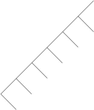
(p1, x1, n1), x1 = 1110

(p4, x4, n4), x4 = 1111

(p5, x5, n5), x5 = 100

(p2, x2, n2), x2 = 10

(p3, x3, n3), x3 = 110

FIGURE 14.3. Assignment of nodes.

In the example, we are able to find nodes at level nk + 1 to which we can assign the triplets. Now we shall prove that there are always enough nodes so that the assignment can be completed. We can perform the assignment of triplets to nodes if and only if the Kraft inequality is satisfied.

We now drop the primes and deal only with the winnowed list illustrated in (14.97). We start with the infinite sum in the Kraft inequality and split it according to the output strings: