

CHAPTER
The z-Transform
33
Just as analog filters are designed using the Laplace transform, recursive digital filters are developed with a parallel technique called the z-transform. The overall strategy of these two transforms is the same: probe the impulse response with sinusoids and exponentials to find the system's poles and zeros. The Laplace transform deals with differential equations, the s-domain, and the s-plane. Correspondingly, the z-transform deals with difference equations, the z-domain, and the z-plane. However, the two techniques are not a mirror image of each other; the s-plane is arranged in a rectangular coordinate system, while the z-plane uses a polar format. Recursive digital filters are often designed by starting with one of the classic analog filters, such as the Butterworth, Chebyshev, or elliptic. A series of mathematical conversions are then used to obtain the desired digital filter. The z-transform provides the framework for this mathematics. The Chebyshev filter design program presented in Chapter 20 uses this approach, and is discussed in detail in this chapter.
The Nature of the z-Domain
To reinforce that the Laplace and z-transforms are parallel techniques, we will start with the Laplace transform and show how it can be changed into the z- transform. From the last chapter, the Laplace transform is defined by the relationship between the time domain and s-domain signals:
4
X (s) ' m x (t ) e & s t d t
t ' & 4
where x (t) and X (s) are the time domain and s-domain representation of the signal, respectively. As discussed in the last chapter, this equation analyzes the time domain signal in terms of sine and cosine waves that have an exponentially changing amplitude. This can be understood by replacing the
605
606 |
The Scientist and Engineer's Guide to Digital Signal Processing |
complex variable, s, with its equivalent expression, F% jT. Using this alternate notation, the Laplace transform becomes:
4
X (F, T) ' m x (t ) e & Ft e & jTt d t
t ' & 4
If we are only concerned with real time domain signals (the usual case), the top and bottom halves of the s-plane are mirror images of each other, and the term, e & jTt , reduces to simple cosine and sine waves. This equation identifies each location in the s-plane by the two parameters, F and T. The value at each location is a complex number, consisting of a real part and an imaginary part. To find the real part, the time domain signal is multiplied by a cosine wave with a frequency of T, and an amplitude that changes exponentially according to the decay parameter, F. The value of the real part of X (F, T) is then equal to the integral of the resulting waveform. The value of the imaginary part of X (F, T) is found in a similar way, except using a sine wave. If this doesn't sound very familiar, you need to review the previous chapter before continuing.
The Laplace transform can be changed into the z-transform in three steps. The first step is the most obvious: change from continuous to discrete signals. This is done by replacing the time variable, t, with the sample number, n, and changing the integral into a summation:
4
X (F, T) ' j x [n] e & Fn e & jTn
n ' & 4
Notice that X (F, T) uses parentheses, indicating it is continuous, not discrete. Even though we are now dealing with a discrete time domain signal, x[n] , the parameters F and T can still take on a continuous range of values. The second step is to rewrite the exponential term. An exponential signal can be mathematically represented in either of two ways:
y [n ] ' e & Fn or |
y [n ] ' r -n |
As illustrated in Fig. 33-1, both these equations generate an exponential curve. The first expression controls the decay of the signal through the parameter, F. If F is positive, the waveform will decrease in value as the sample number, n, becomes larger. Likewise, the curve will progressively increase if F is negative. If F is exactly zero, the signal will have a constant value of one.
FIGURE 33-1
Exponential signals. Exponentials can be represented in two different mathematical forms. The Laplace transform uses one way, while the z-transform uses the other.
Chapter 33The z-Transform |
|
|
|
|
|
|
|
|
|
|
|
607 |
||||||||||||
|
|
|
|
|
|
|
|
|
|
|
|
|
|
|
|
|
|
|
|
|
|
|
|
|
|
a. Decreasing |
|
|
3 |
|
|
|
|
|
|
|
|
|
|
|
|
|
|
|
|
|
|
|
|
|
y [n] ' e & Fn, F ' 0.105 |
2 |
|
|
|
|
|
|
|
|
|
|
|
|
|
|
|
|
|
|
|
|||
|
or |
|
y[n] |
1 |
|
|
|
|
|
|
|
|
|
|
|
|
|
|
|
|
|
|
|
|
|
|
|
|
|
|
|
|
|
|
|
|
|
|
|
|
|
|
|
|
|
|
|||
|
y [n] ' r-n, |
r ' 1.1 |
0 |
|
|
|
|
|
|
|
|
|
|
|
|
|
|
|
|
|
|
|
||
|
|
|
|
|
|
|
|
|
|
|
|
|
|
|
|
|
|
|
|
|
|
|
|
|
|
|
|
|
|
|
|
|
|
|
|
|
|
|
|
|
|
|
|
|
|
|
|
|
|
|
|
|
|
|
-10 |
|
-5 |
0 |
5 |
10 |
||||||||||||||
|
|
|
|
|
|
|
|
|
|
|
|
n |
|
|
|
|
|
|
|
|
|
|
|
|
|
|
|
|
|
|
|
|
|
|
|
|
|
|
|
|
|
|
|
|
|
|
|
|
|
|
b. Constant |
|
|
|
3 |
|
|
|
|
|
|
|
|
|
|
|
|
|
|
|
|
|
|
|
|
|
|
|
|
|
|
|
|
|
|
|
|
|
|
|
|
|
|
|
|
|
|
|
|
|
y [n] ' e & Fn, F ' 0.000 |
2 |
|
|
|
|
|
|
|
|
|
|
|
|
|
|
|
|
|
|
|
|||
|
|
|
|
|
|
|
|
|
|
|
|
|
|
|
|
|
|
|
|
|||||
|
|
|
|
|
|
|
|
|
|
|
|
|
|
|
|
|
|
|
|
|||||
|
|
|
|
|
|
|
|
|
|
|
|
|
|
|
|
|
|
|
|
|||||
|
|
|
|
|
|
|
|
|
|
|
|
|
|
|
|
|
|
|
|
|||||
|
|
|
|
|
|
|
|
|
|
|
|
|
|
|
|
|
|
|
|
|||||
|
or |
|
y[n] |
1 |
|
|
|
|
|
|
|
|
|
|
|
|
|
|
|
|
|
|
|
|
|
|
|
|
|
|
|
|
|
|
|
|
|
|
|
|
|
|
|
|
|
||||
|
|
|
|
|
|
|
|
|
|
|
|
|
|
|
|
|
|
|
|
|
||||
|
|
|
|
|
|
|
|
|
|
|
|
|
|
|
|
|
|
|
|
|
|
|||
|
y [n] ' r-n, |
r ' 1.0 |
|
|
|
|
|
|
|
|
|
|
|
|
|
|
|
|
|
|
|
|||
|
|
|
|
|
|
|
|
|
|
|
|
|
|
|
|
|
|
|
|
|||||
|
|
|
|
|
|
|
|
|
|
|
|
|
|
|
|
|
|
|
|
|||||
|
0 |
|
|
|
|
|
|
|
|
|
|
|
|
|
|
|
|
|
|
|
||||
|
|
|
|
|
|
|
|
|
|
|
|
|
|
|
|
|
|
|
|
|||||
|
|
|
|
|
|
|
|
|
|
|
|
|
|
|
|
|
|
|
|
|
|
|
|
|
|
|
|
|
|
|
|
|
|
|
|
|
|
|
|
|
|
|
|
|
|
|
|
|
|
|
|
|
|
|
|
|
|
|
|
|
|
|
|
|
|
|
|
|
|
|
|
|
|
|
|
|
|
|
|
|
|
|
|
|
|
|
|
|
|
|
|
|
|
|
|
|
|
|
|
|
|
|
|
|
-10 |
|
-5 |
0 |
5 |
10 |
||||||||||||||
n
c. Increasing |
3 |
|
|
|
|
|
|
|
|
|
|
|
|
|
|
|
|
|
|
|
|
|
|
y [n] ' e & Fn, F ' & 0.095 2 


or |
y[n] |
|
|
y [n] ' r-n, r ' 0.9 |
1 |
|
|
|
0 |
-10 |
-5 |
0 |
5 |
10 |
n
The second expression uses the parameter, r, to control the decay of the waveform. The waveform will decrease if r > 1 , and increase if r < 1. The signal will have a constant value when r ' 1 . These two equations are just different ways of expressing the same thing. One method can be swapped for the other by using the relation:
r-n ' [ e ln ( r ) ]-n ' e-n ln ( r ) ' e & Fn
where: F ' ln ( r )
The second step of converting the Laplace transform into the z-transform is completed by using the other exponential form:
4
X (r, T) ' j x [n ] r-n e & jTn
n ' & 4
While this is a perfectly correct expression of the z-transform, it is not in the most compact form for complex notation. This problem was overcome
608 |
The Scientist and Engineer's Guide to Digital Signal Processing |
in the Laplace transform by introducing a new complex variable, s, defined to be: s ' F% jT. In this same way, we will define a new variable for the z- transform:
z ' r e jT
This is defining the complex variable, z, as the polar notation combination of the two real variables, r and T. The third step in deriving the z-transform is to replace: r and T, with z. This produces the standard form of the z- transform:
EQUATION 33-1
The z-transform. The z-transform defines the relationship between the time domain signal, x [n], and the z-domain signal, X (z).
4
X (z) ' j x [n ] z & n
n ' & 4
Why does the z-transform use r n instead of e & Fn , and z instead of s? As described in Chapter 19, recursive filters are implemented by a set of recursion coefficients. To analyze these systems in the z-domain, we must be able to convert these recursion coefficients into the z-domain transfer function, and back again. As we will show shortly, defining the z-transform in this manner ( r n and z) provides the simplest means of moving between these two important representations. In fact, defining the z-domain in this way makes it trivial to move from one representation to the other.
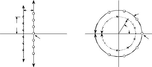
Figure 33-2 illustrates the difference between the Laplace transform's s-plane, and the z-transform's z-plane. Locations in the s-plane are identified by two parameters: F, the exponential decay variable along the horizontal axis, and T, the frequency variable along the vertical axis. In other words, these two real parameters are arranged in a rectangular coordinate system. This geometry results from defining s, the complex variable representing position in the s- plane, by the relation: s ' F% jT.
In comparison, the z-domain uses the variables: r and T, arranged in polar coordinates. The distance from the origin, r, is the value of the exponential decay. The angular distance measured from the positive horizontal axis, T, is the frequency. This geometry results from defining z by: z ' r e & jT . In other words, the complex variable representing position in the z-plane is formed by combining the two real parameters in a polar form.
These differences result in vertical lines in the s-plane matching circles in the z-plane. For example, the s-plane in Fig. 33-2 shows a pole-zero pattern where all of the poles & zeros lie on vertical lines. The equivalent poles & zeros in the z-plane lie on circles concentric with the origin. This can be understood by examining the relation presented earlier: F' & ln(r) . For instance, the s-plane's vertical axis (i.e., F' 0 ) corresponds to the z-plane's
Chapter 33The z-Transform |
609 |
|
s - Plane |
z - Plane |
|
Im |
Im |
|
|
||
F |
|
|
|
r ' 1 |
|
T |
r |
|
T |
||
Re |
||
Re |
||
DC |
DC |
|
( F ' 0, T' 0 ) |
(r ' 1, T' 0 ) |
FIGURE 33-2
Relationship between the s-plane and the z-plane. The s-plane is a rectangular coordinate system with F expressing the distance along the real (horizontal) axis, and T the distance along the imaginary (vertical) axis. In comparison, the z-plane is in polar form, with r being the distance to the origin, and T the angle measured to the positive horizontal axis. Vertical lines in the s-plane, such as illustrated by the example poles and zeros in this figure, correspond to circles in the z-plane.
unit circle (that is, r ' 1 ). Vertical lines in the left half of the s-plane correspond to circles inside the z-plane's unit circle. Likewise, vertical lines in the right half of the s-plane match with circles on the outside of the z-plane's unit circle. In other words, the left and right sides of the s-plane correspond to the interior and the exterior of the unit circle, respectively. For instance, a continuous system is unstable when poles occupy the right half of the s-plane. In this same way, a discrete system is unstable when poles are outside the unit circle in the z-plane. When the time domain signal is completely real (the most common case), the upper and lower halves of the z-plane are mirror images of each other, just as with the s- domain.
Pay particular attention to how the frequency variable, T, is used in the two transforms. A continuous sinusoid can have any frequency between DC and infinity. This means that the s-plane must allow T to run from negative to positive infinity. In comparison, a discrete sinusoid can only have a frequency between DC and one-half the sampling rate. That is, the frequency must be between 0 and 0.5 when expressed as a fraction of the sampling rate, or between 0 and B when expressed as a natural frequency (i.e., T ' 2Bf ). This matches the geometry of the z-plane when we interpret T to be an angle expressed in radians. That is, the positive frequencies correspond to angles of 0 to B radians, while the negative frequencies correspond to 0 to -B radians. Since the z-plane express frequency in a different way than the s-plane, some authors use different symbols to
610 |
The Scientist and Engineer's Guide to Digital Signal Processing |
distinguish the two. A common notation is to use S (an upper case omega) to represent frequency in the z-domain, and T (a lower case omega) for frequency in the s-domain. In this book we will use T to represent both types of frequency, but look for this in other DSP material.
In the s-plane, the values that lie along the vertical axis are equal to the frequency response of the system. That is, the Laplace transform, evaluated at F' 0 , is equal to the Fourier transform. In an analogous manner, the frequency response in the z-domain is found along the unit circle. This can be seen by evaluating the z-transform (Eq. 33-1) at r ' 1 , resulting in the equation reducing to the Discrete Time Fourier Transform (DTFT). This places zero frequency (DC) at a value of one on the horizontal axis in the s-plane. The spectrum's positive frequencies are positioned in a counter-clockwise pattern from this DC position, occupying the upper semicircle. Likewise the negative frequencies are arranged from the DC position along the clockwise path, forming the lower semicircle. The positive and negative frequencies in the spectrum meet at the common point of T ' B and T ' & B. This circular geometry also corresponds to the frequency spectrum of a discrete signal being periodic. That is, when the frequency angle is increased beyond B, the same values are encountered as between 0 and B. When you run around in a circle, you see the same scenery over and over.
Analysis of Recursive Systems
As outlined in Chapter 19, a recursive filter is described by a difference equation:
EQUATION 33-2
Difference equation. See Chapter 19 for details.
y [n ] ' a0 x [n ] % a1 x [n & 1] % a2 x [n & 2] % þ % b1 y [n & 1] % b2 y [n & 2] % b3 y [n & 3] % þ
where x [ ] and y [ ] are the input and output signals, respectively, and the "a" and "b" terms are the recursion coefficients. An obvious use of this equation is to describe how a programmer would implement the filter. An equally important aspect is that it represents a mathematical relationship between the input and output that must be continually satisfied. Just as continuous systems are controlled by differential equations, recursive discrete systems operate in accordance with this difference equation. From this relationship we can derive the key characteristics of the system: the impulse response, step response, frequency response, pole-zero plot, etc.
We start the analysis by taking the z-transform (Eq. 33-1) of both sides of Eq. 33-2. In other words, we want to see what this controlling relationship looks like in the z-domain. With a fair amount of algebra, we can separate the relation into: Y [z] / X [z] , that is, the z-domain representation of the output signal divided by the z-domain representation of the input signal. Just as with

Chapter 33The z-Transform |
611 |
the Laplace transform, this is called the system's transfer function, and designate it by H [z]. Here is what we find:
EQUATION 33-3
Transfer function in polynomial form. The recursion coefficients are directly identifiable in this relation.
|
a |
0 |
% a |
1 |
z & 1 % a |
z & 2 % a |
3 |
z & 3 % þ |
H [z ] ' |
|
|
2 |
|
|
|||
|
|
|
|
|
|
|
|
1 & b1 z & 1 & b2 z & 2 & b3 z & 3 & þ
This is one of two ways that the transfer function can be written. This form is important because it directly contains the recursion coefficients. For example, suppose we know the recursion coefficients of a digital filter, such as might be provided from a design table:
a0 = |
0.389 |
|
|
|
|
a1 |
= -1.558 |
b1 |
= |
2.161 |
|
a2 |
= |
2.338 |
b2 |
= -2.033 |
|
a3 |
= -1.558 |
b3 |
= |
0.878 |
|
a4 |
= |
0.389 |
b4 |
= -0.161 |
|
Without having to worry about nasty complex algebra, we can directly write down the system's transfer function:
H [z ] ' |
0.389 & 1.558 z & 1 % 2.338 z & 2 |
& 1.558 z & 3 % 0.389 z & 4 |
|
|
1 & 2.161 z & 1 % 2.033 z & 2 & 0.878 z & 3 % 0.161 z & 4
Notice that the "b" coefficients enter the transfer function with a negative sign in front of them. Alternatively, some authors write this equation using additions, but change the sign of all the "b" coefficients. Here's the problem. If you are given a set of recursion coefficients (such as from a table or filter design program), there is a 50-50 chance that the "b" coefficients will have the opposite sign from what you expect. If you don't catch this discrepancy, the filter will be grossly unstable.
Equation 33-3 expresses the transfer function using negative powers of z, such as: z & 1, z & 2, z & 3, etc. After an actual set of recursion coefficients have been plugged in, we can convert the transfer function into a more conventional form that uses positive powers: i.e., z, z 2, z 3, þ. By multiplying both the numerator and denominator of our example by z 4 , we obtain:
H [z ] ' |
0.389 z 4 |
& 1.558 z 3 % 2.338 z 2 & 1.558 z % 0.389 |
|
|
z 4 & 2.161 z 3 % 2.033 z 2 & 0.878 z % 0.161

612 |
The Scientist and Engineer's Guide to Digital Signal Processing |
Positive powers are often easier to use, and they are required by some z- domain techniques. Why not just rewrite Eq. 33-3 using positive powers and forget about negative powers entirely? We can't! The trick of multiplying the numerator and denominator by the highest power of z (such as z 4 in our example) can only be used if the number of recursion coefficients is already known. Equation 33-3 is written for an arbitrary number of coefficients. The point is, both positive and negative powers are routinely used in DSP and you need to know how to convert between the two forms.
The transfer function of a recursive system is useful because it can be manipulated in ways that the recursion coefficients cannot. This includes such tasks as: combining cascade and parallel stages into a single system, designing filters by specifying the pole and zero locations, converting analog filters into digital, etc. These operations are carried out by algebra performed in the z- domain, such as: multiplication, addition, and factoring. After these operations are completed, the transfer function is placed in the form of Eq. 33-3, allowing the new recursion coefficients to be identified.
Just as with the s-domain, an important feature of the z-domain is that the transfer function can be expressed as poles and zeros. This provides the second general form of the z-domain:
EQUATION 33-4 |
H [z ] ' |
(z & z |
1) (z & z2) (z & z3)þ |
|
Transfer function in pole-zero form. |
|
|
||
(z & p1) (z & p2) (z & p3)þ |
||||
|
|
|||
Each of the poles (p1, p2, p3, þ) and zeros ( z1, z2, z3 þ) is a complex number. To move from Eq. 33-4 to 33-3, multiply out the expressions and collect like terms. While this can involve a tremendous amount of algebra, it is straightforward in principle and can easily be written into a computer routine. Moving from Eq. 33-3 to 33-4 is more difficult because it requires factoring of the polynomials. As discussed in Chapter 32, the quadratic equation can be used for the factoring if the transfer function is second order or less (i.e., there are no powers of z higher than z 2). Algebraic methods cannot generally be used to factor systems greater than second order and numerical methods must be employed. Fortunately, this is seldom needed; digital filter design starts with the pole-zero locations (Eq. 33-4) and ends with the recursion coefficients (Eq. 33-3), not the other way around.
As with all complex numbers, the pole and zero locations can be represented in either polar or rectangular form. Polar notation has the advantage of being more consistent with the natural organization of the z-plane. In comparison, rectangular form is generally preferred for mathematical work, that is, it is usually easier to manipulate: F% jT, as compared with: r e jT .
As an example of using these equations, we will design a notch filter by the following steps: (1) specify the pole-zero placement in the z-plane, (2)
Chapter 33The z-Transform |
613 |
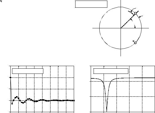
FIGURE 33-3
Notch filter designed in the z-domain. The design starts by locating two poles and two zeros in the z-plane, as shown in (a). The resulting impulse and frequency response are shown in (b) and (c), respectively. The sharpness of the notch is controlled by the distance of the poles from the zeros.
1.5
b. Impulse response
|
1.0 |
|
|
|
|
|
|
|
|
Amplitude |
0.5 |
|
|
|
|
|
|
|
|
|
|
|
|
|
|
|
|
|
|
|
0.0 |
|
|
|
|
|
|
|
|
|
-0.5 |
|
|
|
|
|
|
|
|
|
0 |
5 |
10 |
15 |
20 |
25 |
30 |
35 |
40 |
Sample number
a. Pole-zero plot |
Im |
|
r ' 0.9 |
||
|
||
|
r ' 1 |
|
|
B/4 |
|
|
Re |
|
1.5 |
|
c. Frequency response
1.0 |
|
|
|
|
|
Amplitude |
|
|
|
|
|
0.5 |
|
|
|
|
|
0.0 |
|
|
|
|
|
0 |
0.1 |
0.2 |
0.3 |
0.4 |
0.5 |
Frequency
write down the transfer function in the form of Eq. 33-4, (3) rearrange the transfer function into the form of Eq. 33-3, and (4) identify the recursion coefficients needed to implement the filter. Fig. 33-3 shows the example we will use: a notch filter formed from two poles and two zeros located at
In polar form: In rectangular form:
z |
1 |
' 1.00 e j (B/4) |
z |
1 |
' 0.7071 % j 0.7071 |
|
|
|
|
||
z |
2 |
' 1.00 e j (& B/4) |
z |
2 |
' 0.7071 & j 0.7071 |
|
|
|
|
||
p |
1 |
' 0.90 e j (B/4) |
p |
1 |
' 0.6364 % j 0.6364 |
|
|
|
|
||
p |
2 |
' 0.90 e j (& B/4) |
p |
2 |
' 0.6364 & j 0.6364 |
|
|
|
|
To understand why this is a notch filter, compare this pole-zero plot with Fig. 32-6, a notch filter in the s-plane. The only difference is that we are moving along the unit circle to find the frequency response from the z-plane, as opposed to moving along the vertical axis to find the frequency response from the s-plane. From the polar form of the poles and zeros, it can be seen that the notch will occur at a natural frequency of B/4 , corresponding to 0.125 of the sampling rate.

614 |
The Scientist and Engineer's Guide to Digital Signal Processing |
Since the pole and zero locations are known, the transfer function can be written in the form of Eq. 33-4 by simply plugging in the values:
H (z) ' |
[ z & (0.7071 % j 0.7071) ] |
[z & (0.7071 & j 0.7071) ] |
|
[ z & (0.6364 % j 0.6364)] |
[ z & (0.6364 & j 0.6364) ] |
||
|
To find the recursion coefficients that implement this filter, the transfer function must be rearranged into the form of Eq. 33-3. To start, expand the expression by multiplying out the terms:
H (z ) ' |
z 2 |
& 0.7071 z % j 0.7071 z & |
0.7071 z % |
0.70712 |
& j 0.70712 |
& j 0.7071 z % j 0.70712 & j 2 0.70712 |
|
z 2 |
& 0.6364 z % j 0.6364 z & |
0.6364 z % |
0.63642 & j 0.63642 |
& j 0.6364 z % j 0.63642 & j 2 0.63642 |
|||
|
|||||||
Next, we collect like terms and reduce. As long as the upper half of the z- plane is a mirror image of the lower half (which is always the case if we are dealing with a real impulse response), all of the terms containing a " j " will cancel out of the expression:
H [z ] ' |
1.000 & 1.414 z % 1.000 z 2 |
|
0.810 & 1.273 z % 1.000 z 2 |
||
|
While this is in the form of one polynomial divided by another, it does not use negative exponents of z, as required by Eq. 33-3. This can be changed by dividing both the numerator and denominator by the highest power of z in the expression, in this case, z 2 :
H [z ] ' |
1.000 & 1.414 z & 1 % 1.000 z & 2 |
|
1.000 & 1.273 z & 1 % 0.810 z & 2 |
||
|
Since the transfer function is now in the form of Eq. 33-3, the recursive coefficients can be directly extracted by inspection:
a0 |
= |
1.000 |
|
|
a1 |
= -1.414 |
b1 |
= 1.273 |
|
a2 |
= |
1.000 |
b2 |
= -0.810 |
This example provides the general strategy for obtaining the recursion coefficients from a pole-zero plot. In specific cases, it is possible to derive