

CHAPTER
The Discrete Fourier Transform
8
Fourier analysis is a family of mathematical techniques, all based on decomposing signals into sinusoids. The discrete Fourier transform (DFT) is the family member used with digitized signals. This is the first of four chapters on the real DFT, a version of the discrete Fourier transform that uses real numbers to represent the input and output signals. The complex DFT, a more advanced technique that uses complex numbers, will be discussed in Chapter 31. In this chapter we look at the mathematics and algorithms of the Fourier decomposition, the heart of the DFT.
The Family of Fourier Transform
Fourier analysis is named after Jean Baptiste Joseph Fourier (1768-1830), a French mathematician and physicist. (Fourier is pronounced: for@¯e@¯a , and is always capitalized). While many contributed to the field, Fourier is honored for his mathematical discoveries and insight into the practical usefulness of the techniques. Fourier was interested in heat propagation, and presented a paper in 1807 to the Institut de France on the use of sinusoids to represent temperature distributions. The paper contained the controversial claim that any continuous periodic signal could be represented as the sum of properly chosen sinusoidal waves. Among the reviewers were two of history's most famous mathematicians, Joseph Louis Lagrange (1736-1813), and Pierre Simon de Laplace (1749-1827).
While Laplace and the other reviewers voted to publish the paper, Lagrange adamantly protested. For nearly 50 years, Lagrange had insisted that such an approach could not be used to represent signals with corners, i.e., discontinuous slopes, such as in square waves. The Institut de France bowed to the prestige of Lagrange, and rejected Fourier's work. It was only after Lagrange died that the paper was finally published, some 15 years later. Luckily, Fourier had other things to keep him busy, political activities, expeditions to Egypt with Napoleon, and trying to avoid the guillotine after the French Revolution (literally!).
141
142 |
The Scientist and Engineer's Guide to Digital Signal Processing |
Who was right? It's a split decision. Lagrange was correct in his assertion that a summation of sinusoids cannot form a signal with a corner. However, you can get very close. So close that the difference between the two has zero energy. In this sense, Fourier was right, although 18th century science knew little about the concept of energy. This phenomenon now goes by the name: Gibbs Effect, and will be discussed in Chapter 11.
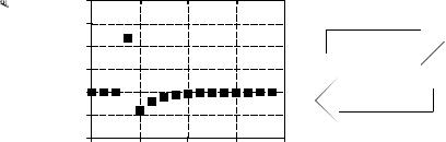
Figure 8-1 illustrates how a signal can be decomposed into sine and cosine waves. Figure (a) shows an example signal, 16 points long, running from sample number 0 to 15. Figure (b) shows the Fourier decomposition of this signal, nine cosine waves and nine sine waves, each with a different frequency and amplitude. Although far from obvious, these 18 sinusoids
FIGURE 8-1a (see facing page)
Amplitude
80 |
|
|
|
|
60 |
|
|
|
|
40 |
|
|
|
|
20 |
|
|
|
|
0 |
|
|
|
|
-20 |
|
|
|
|
-40 |
|
|
|
|
0 |
4 |
8 |
12 |
16 |
Sample number
DECOMPOSE
SYNTHESIZE
add to produce the waveform in (a). It should be noted that the objection made by Lagrange only applies to continuous signals. For discrete signals, this decomposition is mathematically exact. There is no difference between the signal in (a) and the sum of the signals in (b), just as there is no difference between 7 and 3+4.
Why are sinusoids used instead of, for instance, square or triangular waves? Remember, there are an infinite number of ways that a signal can be decomposed. The goal of decomposition is to end up with something easier to deal with than the original signal. For example, impulse decomposition allows signals to be examined one point at a time, leading to the powerful technique of convolution. The component sine and cosine waves are simpler than the original signal because they have a property that the original signal does not have: sinusoidal fidelity. As discussed in Chapter 5, a sinusoidal input to a system is guaranteed to produce a sinusoidal output. Only the amplitude and phase of the signal can change; the frequency and wave shape must remain the same. Sinusoids are the only waveform that have this useful property. While square and triangular decompositions are possible, there is no general reason for them to be useful.
The general term: Fourier transform, can be broken into four categories, resulting from the four basic types of signals that can be encountered.
Chapter 8- The Discrete Fourier Transform |
143 |
Cosine Waves
8 4 


0 


 -4
-4 


 -8
-8 


0 |
2 |
4 |
6 |
8 |
10 |
12 |
14 |
16 |
8 |
|
|
|
|
|
|
|
|
4 |
|
|
|
|
|
|
|
|
0 |
|
|
|
|
|
|
|
|
-4 |
|
|
|
|
|
|
|
|
-8 |
|
|
|
|
|
|
|
|
0 |
2 |
4 |
6 |
8 |
10 |
12 |
14 |
16 |
8 |
|
|
|
|
|
|
|
|
4 |
|
|
|
|
|
|
|
|
0 |
|
|
|
|
|
|
|
|
-4 |
|
|
|
|
|
|
|
|
-8 |
|
|
|
|
|
|
|
|
0 |
2 |
4 |
6 |
8 |
10 |
12 |
14 |
16 |
8 |
|
|
|
|
|
|
|
|
4 |
|
|
|
|
|
|
|
|
0 |
|
|
|
|
|
|
|
|
-4 |
|
|
|
|
|
|
|
|
-8 |
|
|
|
|
|
|
|
|
0 |
2 |
4 |
6 |
8 |
10 |
12 |
14 |
16 |
8 4 


0 


 -4
-4 


 -8
-8 


0 |
2 |
4 |
6 |
8 |
10 |
12 |
14 |
16 |
8 |
|
|
|
|
|
|
|
|
4 |
|
|
|
|
|
|
|
|
0 |
|
|
|
|
|
|
|
|
-4 |
|
|
|
|
|
|
|
|
-8 |
|
|
|
|
|
|
|
|
0 |
2 |
4 |
6 |
8 |
10 |
12 |
14 |
16 |
8 4 


0 


 -4
-4 


 -8
-8 


0 |
2 |
4 |
6 |
8 |
10 |
12 |
14 |
16 |
8 |
|
|
|
|
|
|
|
|
4 |
|
|
|
|
|
|
|
|
0 |
|
|
|
|
|
|
|
|
-4 |
|
|
|
|
|
|
|
|
-8 |
|
|
|
|
|
|
|
|
0 |
2 |
4 |
6 |
8 |
10 |
12 |
14 |
16 |
8 |
|
|
|
|
|
|
|
|
4 |
|
|
|
|
|
|
|
|
0 |
|
|
|
|
|
|
|
|
-4 |
|
|
|
|
|
|
|
|
-8 |
|
|
|
|
|
|
|
|
0 |
2 |
4 |
6 |
8 |
10 |
12 |
14 |
16 |
Sine Waves
8 4 


0 


 -4
-4 


-8 


 0 2 4 6 8 10 12 14 16
8 4 


0 


 -4
-4 


 -8
-8 


0 |
2 |
4 |
6 |
8 |
10 |
12 |
14 |
16 |
8 |
|
|
|
|
|
|
|
|
4 |
|
|
|
|
|
|
|
|
0 |
|
|
|
|
|
|
|
|
-4 |
|
|
|
|
|
|
|
|
-8 |
|
|
|
|
|
|
|
|
0 |
2 |
4 |
6 |
8 |
10 |
12 |
14 |
16 |
8 |
|
|
|
|
|
|
|
|
4 |
|
|
|
|
|
|
|
|
0 |
|
|
|
|
|
|
|
|
-4 |
|
|
|
|
|
|
|
|
-8 |
|
|
|
|
|
|
|
|
0 |
2 |
4 |
6 |
8 |
10 |
12 |
14 |
16 |
8 |
|
|
|
|
|
|
|
|
4 |
|
|
|
|
|
|
|
|
0 |
|
|
|
|
|
|
|
|
-4 |
|
|
|
|
|
|
|
|
-8 |
|
|
|
|
|
|
|
|
0 |
2 |
4 |
6 |
8 |
10 |
12 |
14 |
16 |
8 |
|
|
|
|
|
|
|
|
4 |
|
|
|
|
|
|
|
|
0 |
|
|
|
|
|
|
|
|
-4 |
|
|
|
|
|
|
|
|
-8 |
|
|
|
|
|
|
|
|
0 |
2 |
4 |
6 |
8 |
10 |
12 |
14 |
16 |
8 |
|
|
|
|
|
|
|
|
4 |
|
|
|
|
|
|
|
|
0 |
|
|
|
|
|
|
|
|
-4 |
|
|
|
|
|
|
|
|
-8 |
|
|
|
|
|
|
|
|
0 |
2 |
4 |
6 |
8 |
10 |
12 |
14 |
16 |
8 |
|
|
|
|
|
|
|
|
4 |
|
|
|
|
|
|
|
|
0 |
|
|
|
|
|
|
|
|
-4 |
|
|
|
|
|
|
|
|
-8 |
|
|
|
|
|
|
|
|
0 |
2 |
4 |
6 |
8 |
10 |
12 |
14 |
16 |
8 4 


0 


 -4
-4 


-8 


 0 2 4 6 8 10 12 14 16
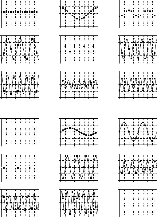
FIGURE 8-1b
Example of Fourier decomposition. A 16 point signal (opposite page) is decomposed into 9 cosine waves and 9 sine waves. The frequency of each sinusoid is fixed; only the amplitude is changed depending on the shape of the waveform being decomposed.
144 |
The Scientist and Engineer's Guide to Digital Signal Processing |
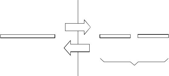
A signal can be either continuous or discrete, and it can be either periodic or aperiodic. The combination of these two features generates the four categories, described below and illustrated in Fig. 8-2.
Aperiodic-Continuous
This includes, for example, decaying exponentials and the Gaussian curve. These signals extend to both positive and negative infinity without repeating in a periodic pattern. The Fourier Transform for this type of signal is simply called the Fourier Transform.
Periodic-Continuous
Here the examples include: sine waves, square waves, and any waveform that repeats itself in a regular pattern from negative to positive infinity. This version of the Fourier transform is called the Fourier Series.
Aperiodic-Discrete
These signals are only defined at discrete points between positive and negative infinity, and do not repeat themselves in a periodic fashion. This type of Fourier transform is called the Discrete Time Fourier Transform.
Periodic-Discrete
These are discrete signals that repeat themselves in a periodic fashion from negative to positive infinity. This class of Fourier Transform is sometimes called the Discrete Fourier Series, but is most often called the Discrete
Fourier Transform.
You might be thinking that the names given to these four types of Fourier transforms are confusing and poorly organized. You're right; the names have evolved rather haphazardly over 200 years. There is nothing you can do but memorize them and move on.
These four classes of signals all extend to positive and negative infinity. Hold on, you say! What if you only have a finite number of samples stored in your computer, say a signal formed from 1024 points. Isn't there a version of the Fourier Transform that uses finite length signals? No, there isn't. Sine and cosine waves are defined as extending from negative infinity to positive infinity. You cannot use a group of infinitely long signals to synthesize something finite in length. The way around this dilemma is to make the finite data look like an infinite length signal. This is done by imagining that the signal has an infinite number of samples on the left and right of the actual points. If all these “imagined” samples have a value of zero, the signal looks discrete and aperiodic, and the Discrete Time Fourier Transform applies. As an alternative, the imagined samples can be a duplication of the actual 1024 points. In this case, the signal looks discrete and periodic, with a period of 1024 samples. This calls for the Discrete Fourier Transform to be used.
As it turns out, an infinite number of sinusoids are required to synthesize a signal that is aperiodic. This makes it impossible to calculate the Discrete Time Fourier Transform in a computer algorithm. By elimination, the only

Chapter 8- The Discrete Fourier Transform |
145 |
|
Type of Transform |
Example Signal |
|
Fourier Transform
signals that are continious and aperiodic
Fourier Series
signals that are continious and periodic
Discrete Time Fourier Transform signals that are discrete and aperiodic
Discrete Fourier Transform signals that are discrete and periodic
FIGURE 8-2
Illustration of the four Fourier transforms. A signal may be continuous or discrete, and it may be periodic or aperiodic. Together these define four possible combinations, each having its own version of the Fourier transform. The names are not well organized; simply memorize them.
type of Fourier transform that can be used in DSP is the DFT. In other words, digital computers can only work with information that is discrete and finite in length. When you struggle with theoretical issues, grapple with homework problems, and ponder mathematical mysteries, you may find yourself using the first three members of the Fourier transform family. When you sit down to your computer, you will only use the DFT. We will briefly look at these other Fourier transforms in future chapters. For now, concentrate on understanding the Discrete Fourier Transform.
Look back at the example DFT decomposition in Fig. 8-1. On the face of it, it appears to be a 16 point signal being decomposed into 18 sinusoids, each consisting of 16 points. In more formal terms, the 16 point signal, shown in (a), must be viewed as a single period of an infinitely long periodic signal. Likewise, each of the 18 sinusoids, shown in (b), represents a 16 point segment from an infinitely long sinusoid. Does it really matter if we view this as a 16 point signal being synthesized from 16 point sinusoids, or as an infinitely long periodic signal being synthesized from infinitely long sinusoids? The answer is: usually no, but sometimes, yes. In upcoming chapters we will encounter properties of the DFT that seem baffling if the signals are viewed as finite, but become obvious when the periodic nature is considered. The key point to understand is that this periodicity is invoked in order to use a mathematical tool, i.e., the DFT. It is usually meaningless in terms of where the signal originated or how it was acquired.

146 |
The Scientist and Engineer's Guide to Digital Signal Processing |
Each of the four Fourier Transforms can be subdivided into real and complex versions. The real version is the simplest, using ordinary numbers and algebra for the synthesis and decomposition. For instance, Fig. 8-1 is an example of the real DFT. The complex versions of the four Fourier transforms are immensely more complicated, requiring the use of complex numbers. These are numbers such as: 3 %4 j , where j is equal to  &1 (electrical engineers use the variable j, while mathematicians use the variable, i). Complex mathematics can quickly become overwhelming, even to those that specialize in DSP. In fact, a primary goal of this book is to present the fundamentals of DSP without the use of complex math, allowing the material to be understood by a wider range of scientists and engineers. The complex Fourier transforms are the realm of those that specialize in DSP, and are willing to sink to their necks in the swamp of mathematics. If you are so inclined, Chapters 30-33 will take you there.
The mathematical term: transform, is extensively used in Digital Signal Processing, such as: Fourier transform, Laplace transform, Z transform, Hilbert transform, Discrete Cosine transform, etc. Just what is a transform? To answer this question, remember what a function is. A function is an algorithm or procedure that changes one value into another value. For example, y ' 2 x %1 is a function. You pick some value for x, plug it into the equation, and out pops a value for y. Functions can also change several values into a single value, such as: y ' 2 a % 3 b % 4 c , where a, b, and c are changed into y.
Transforms are a direct extension of this, allowing both the input and output to have multiple values. Suppose you have a signal composed of 100 samples. If you devise some equation, algorithm, or procedure for changing these 100 samples into another 100 samples, you have yourself a transform. If you think it is useful enough, you have the perfect right to attach your last name to it and expound its merits to your colleagues. (This works best if you are an eminent 18th century French mathematician). Transforms are not limited to any specific type or number of data. For example, you might have 100 samples of discrete data for the input and 200 samples of discrete data for the output. Likewise, you might have a continuous signal for the input and a continuous signal for the output. Mixed signals are also allowed, discrete in and continuous out, and vice versa. In short, a transform is any fixed procedure that changes one chunk of data into another chunk of data. Let's see how this applies to the topic at hand: the Discrete Fourier transform.
Notation and Format of the Real DFT
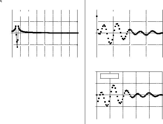
As shown in Fig. 8-3, the discrete Fourier transform changes an N point input signal into two N/2 %1 point output signals. The input signal contains the signal being decomposed, while the two output signals contain the amplitudes of the component sine and cosine waves (scaled in a way we will discuss shortly). The input signal is said to be in the time domain. This is because the most common type of signal entering the DFT is composed of
Chapter 8- The Discrete Fourier Transform |
147 |
|
Time Domain |
Frequency Domain |
|
|
|
|
|
|
|
x[ ] |
|
|
|
|
Forward DFT |
|
|
Re X[ ] |
|
|
Im X[ ] |
||||||||||||||||
|
|
|
|
|
|
|
|
|
|
|
|
|
|
|
|||||||||||||||||||
|
|
|
|
|
|
|
|
|
|
|
|
|
|
|
|
|
|
|
|
|
|
|
|
|
|
|
|
|
|
|
|
|
|
|
|
|
|
|
|
|
|
|
|
|
|
|
|
|
|
|
|
|
|
|
|
|
|
|
|
|
|
|
|
|
|
|
|
0 |
|
|
|
|
N samples |
|
|
|
N-1 |
0 |
|
|
|
|
|
|
N/2 |
0 |
|
|
|
|
|
|
N/2 |
||||||||
|
|
|
|
|
|
|
|
|
|
|
N/2+1 samples |
|
N/2+1 samples |
||||||||||||||||||||
|
|
|
|
|
|
|
|
|
|
|
|
|
|
|
Inverse DFT |
|
|
||||||||||||||||
|
|
|
|
|
|
|
|
|
|
|
|
|
|
|
(cosine wave amplitudes) |
(sine wave amplitudes) |
|||||||||||||||||
collectively referred to as X[ ]
FIGURE 8-3
DFT terminology. In the time domain, x[ ] consists of N points running from 0 to N& 1 . In the frequency domain, the DFT produces two signals, the real part, written: Re X [ ], and the imaginary part, written: Im X [ ]. Each of these frequency domain signals are N/2 % 1 points long, and run from 0 to N/2 . The Forward DFT transforms from the time domain to the frequency domain, while the Inverse DFT transforms from the frequency domain to the time domain. (Take note: this figure describes the real DFT. The complex DFT, discussed in Chapter 31, changes N complex points into another set of N complex points).
samples taken at regular intervals of time. Of course, any kind of sampled data can be fed into the DFT, regardless of how it was acquired. When you see the term "time domain" in Fourier analysis, it may actually refer to samples taken over time, or it might be a general reference to any discrete signal that is being decomposed. The term frequency domain is used to describe the amplitudes of the sine and cosine waves (including the special scaling we promised to explain).
The frequency domain contains exactly the same information as the time domain, just in a different form. If you know one domain, you can calculate the other. Given the time domain signal, the process of calculating the frequency domain is called decomposition, analysis, the forward DFT, or simply, the DFT. If you know the frequency domain, calculation of the time domain is called synthesis, or the inverse DFT. Both synthesis and analysis can be represented in equation form and computer algorithms.
The number of samples in the time domain is usually represented by the variable N. While N can be any positive integer, a power of two is usually chosen, i.e., 128, 256, 512, 1024, etc. There are two reasons for this. First, digital data storage uses binary addressing, making powers of two a natural signal length. Second, the most efficient algorithm for calculating the DFT, the Fast Fourier Transform (FFT), usually operates with N that is a power of two. Typically, N is selected between 32 and 4096. In most cases, the samples run from 0 to N&1 , rather than 1 to N.
Standard DSP notation uses lower case letters to represent time domain signals, such as x[ ] , y[ ] , and z[ ] . The corresponding upper case letters are
148 |
The Scientist and Engineer's Guide to Digital Signal Processing |
|
|
used to represent their frequency domains, that is, X [ ], Y [ ], and |
Z [ ]. For |
|
illustration, assume an N point time domain signal is contained in |
x[ ] . The |
frequency domain of this signal is called X [ ], and consists of two parts, each an array of N/2 %1 samples. These are called the Real part of X [ ] , written as: Re X [ ], and the Imaginary part of X [ ] , written as: Im X [ ]. The values in Re X [ ] are the amplitudes of the cosine waves, while the values in Im X [ ] are the amplitudes of the sine waves (not worrying about the scaling factors for the moment). Just as the time domain runs from x[0] to x[N&1] , the frequency domain signals run from Re X[0] to Re X[N/2], and from Im X[0] to Im X [N/2]. Study these notations carefully; they are critical to understanding the equations in DSP. Unfortunately, some computer languages don't distinguish between lower and upper case, making the variable names up to the individual programmer. The programs in this book use the array XX[ ] to hold the time domain signal, and the arrays REX[ ] and IMX[ ] to hold the frequency domain signals.
The names real part and imaginary part originate from the complex DFT, where they are used to distinguish between real and imaginary numbers. Nothing so complicated is required for the real DFT. Until you get to Chapter 31, simply think that "real part" means the cosine wave amplitudes, while "imaginary part" means the sine wave amplitudes. Don't let these suggestive names mislead you; everything here uses ordinary numbers.
Likewise, don't be misled by the lengths of the frequency domain signals. It is common in the DSP literature to see statements such as: "The DFT changes an N point time domain signal into an N point frequency domain signal." This is referring to the complex DFT, where each "point" is a complex number (consisting of real and imaginary parts). For now, focus on learning the real DFT, the difficult math will come soon enough.
The Frequency Domain's Independent Variable
Figure 8-4 shows an example DFT with N ' 128 . The time domain signal is contained in the array: x[0] to x[127] . The frequency domain signals are contained in the two arrays: Re X[0] to Re X[64] , and Im X [0] to Im X [64]. Notice that 128 points in the time domain corresponds to 65 points in each of the frequency domain signals, with the frequency indexes running from 0 to 64. That is, N points in the time domain corresponds to N/2 %1 points in the frequency domain (not N/2 points). Forgetting about this extra point is a common bug in DFT programs.
The horizontal axis of the frequency domain can be referred to in four different ways, all of which are common in DSP. In the first method, the horizontal axis is labeled from 0 to 64, corresponding to the 0 to N/2 samples in the arrays. When this labeling is used, the index for the frequency domain is an integer, for example, Re X [k] and Im X [k], where k runs from 0 to N/2 in steps of one. Programmers like this method because it is how they write code, using an index to access array locations. This notation is used in Fig. 8-4b.
|
|
|
|
|
|
|
|
|
|
Chapter 8- The Discrete Fourier Transform |
149 |
||||||||||||
|
|
|
|
|
Time Domain |
|
|
|
|
|
Frequency Domain |
|
|
||||||||||
2 |
|
|
|
|
|
|
|
|
|
|
8 |
|
|
|
|
|
|
|
|
|
|
|
|
|
|
|
|
|
|
|
|
|
|
|
|
|
|
|
|
|
|
|
|
|
|
||
|
|
|
|
|
|
|
|
|
|
|
|
|
|
|
|
|
|
|
|
||||
|
|
|
|
|
a. x[ ] |
|
|
|
|
|
|
|
|
|
b. Re X[ ] |
|
|
|
|||||
1 |
|
|
|
|
|
|
|
|
|
|
4 |
|
|
|
|
|
|
|
|
|
|
|
|
|
|
|
|
|
|
|
|
|
|
|
|
|
|
|
|
|
|
|
|
|
|
||
Amplitude |
0 |
Amplitude |
0 |
|
|
-1 |
|
|
|
|
|
|
|
|
|
|
|
|
|
|
|
|
|
|
|
|
|
|
|
|
|
|
|
-4 |
|
|
|
|
|
|
|
|
|
|
|
|
|
|
-2 |
|
|
|
|
|
|
|
|
|
|
|
|
|
|
|
|
|
|
|
|
|
|
|
|
|
|
|
-8 |
|
|
|
|
|
|
|
|
|
|
|
|
|
|
0 |
16 |
32 |
48 |
64 |
80 |
96 |
112 |
1287 |
0 |
16 |
32 |
48 |
64 |
|||||||||||||||||||||||||||||
|
|
|
|
|
|
|
|
|
|
Sample number |
|
|
|
|
|
|
|
|
|
|
|
|
Frequency (sample number) |
|
|
|||||||||||||||||
FIGURE 8-4 |
|
|
8 |
Example of the DFT. The DFT converts the |
|
c. Im X[ ] |
|
time domain signal, x[ ], into the frequency |
|
|
|
domain signals, Re X [ ] a n d Im X [ ]. |
The |
|
4 |
horizontal axis of the frequency domain can be |
Amplitude |
|
|
labeled in one of three ways: (1) as an array |
|
||
|
|
||
index that runs between 0 and N/2 , (2) as a |
|
0 |
|
fraction of the sampling frequency, running |
|
|
|
between 0 and 0.5, (3) as a natural frequency, |
|
|
|
running between 0 and B. In the example |
|
-4 |
|
shown here, (b) uses the first method, while (c) |
|
|
|
use the second method. |
|
|
|
-8 |
|
|
|
|
|
|
|
|
|
|
|
|
|
|
|
0 |
0.1 |
0.2 |
0.3 |
0.4 |
0.5 |
||||||||||
|
|
Frequency (fraction of sampling rate) |
|
|
|||||||||||
In the second method, used in (c), the horizontal axis is labeled as a fraction of the sampling rate. This means that the values along the horizonal axis always run between 0 and 0.5, since discrete data can only contain frequencies between DC and one-half the sampling rate. The index used with this notation is f, for frequency. The real and imaginary parts are written: Re X [f ] and Im X [f ], where f takes on N/2 %1 equally spaced values between 0 and 0.5. To convert from the first notation, k, to the second notation, f , divide the horizontal axis by N. That is, f ' k/N . Most of the graphs in this book use this second method, reinforcing that discrete signals only contain frequencies between 0 and 0.5 of the sampling rate.
The third style is similar to the second, except the horizontal axis is multiplied by 2B. The index used with this labeling is T, a lower case Greek omega. In this notation, the real and imaginary parts are written: Re X [T] and Im X [T], where T takes on N/2 %1 equally spaced values between 0 and B. The parameter, T, is called the natural frequency, and has the units of radians. This is based on the idea that there are 2B radians in a circle. Mathematicians like this method because it makes the equations shorter. For instance, consider how a cosine wave is written in each of
t h e s e f i r s t t h r e e n o t a t i o n s : |
u s i n g k : c [n ] ' cos (2Bkn / N) , u s i n g f : |
c [n ] ' cos (2Bfn ) , and using T: |
c [n ] ' cos (Tn ) . |
150 |
The Scientist and Engineer's Guide to Digital Signal Processing |
The fourth method is to label the horizontal axis in terms of the analog frequencies used in a particular application. For instance, if the system being examined has a sampling rate of 10 kHz (i.e., 10,000 samples per second), graphs of the frequency domain would run from 0 to 5 kHz. This method has the advantage of presenting the frequency data in terms of a real world meaning. The disadvantage is that it is tied to a particular sampling rate, and is therefore not applicable to general DSP algorithm development, such as designing digital filters.
All of these four notations are used in DSP, and you need to become comfortable with converting between them. This includes both graphs and mathematical equations. To find which notation is being used, look at the independent variable and its range of values. You should find one of four notations: k (or some other integer index), running from 0 to N/2 ; f, running from 0 to 0.5; T, running from 0 to B; or a frequency expressed in hertz, running from DC to one-half of an actual sampling rate.
DFT Basis Functions
The sine and cosine waves used in the DFT are commonly called the DFT basis functions. In other words, the output of the DFT is a set of numbers that represent amplitudes. The basis functions are a set of sine and cosine waves with unity amplitude. If you assign each amplitude (the frequency domain) to the proper sine or cosine wave (the basis functions), the result is a set of scaled sine and cosine waves that can be added to form the time domain signal.
The DFT basis functions are generated from the equations:
EQUATION 8-1
Equations for the DFT basis functions. In these equations, ck[ i] and sk[ i] are the cosine and sine waves, each N points in length, running from i ' 0 to N& 1 . The parameter, k, determines the frequency of the wave. In an N point DFT, k takes on values between 0 and N/2 .
ck [i ] ' cos ( 2Bki / N ) sk [i ] ' sin ( 2Bki / N )
where: ck[ ] is the cosine wave for the amplitude held in Re X[k] , and sk[ ] is the sine wave for the amplitude held in Im X [k]. For example, Fig. 8-5 shows some of the 17 sine and 17 cosine waves used in an N ' 32 point DFT. Since these sinusoids add to form the input signal, they must be the same length as the input signal. In this case, each has 32 points running from i ' 0 to 31. The parameter, k, sets the frequency of each sinusoid. In particular, c1[ ] is the cosine wave that makes one complete cycle in N points, c5[ ] is the cosine wave that makes five complete cycles in N points, etc. This is an important concept in understanding the basis functions; the frequency parameter, k, is equal to the number of complete cycles that occur over the N points of the signal.