

CHAPTER
Linear Systems
5
Most DSP techniques are based on a divide-and-conquer strategy called superposition. The signal being processed is broken into simple components, each component is processed individually, and the results reunited. This approach has the tremendous power of breaking a single complicated problem into many easy ones. Superposition can only be used with linear systems, a term meaning that certain mathematical rules apply. Fortunately, most of the applications encountered in science and engineering fall into this category. This chapter presents the foundation of DSP: what it means for a system to be linear, various ways for breaking signals into simpler components, and how superposition provides a variety of signal processing techniques.
Signals and Systems
A signal is a description of how one parameter varies with another parameter. For instance, voltage changing over time in an electronic circuit, or brightness varying with distance in an image. A system is any process that produces an output signal in response to an input signal. This is illustrated by the block diagram in Fig. 5-1. Continuous systems input and output continuous signals, such as in analog electronics. Discrete systems input and output discrete signals, such as computer programs that manipulate the values stored in arrays.
Several rules are used for naming signals. These aren't always followed in DSP, but they are very common and you should memorize them. The mathematics is difficult enough without a clear notation. First, continuous signals use parentheses, such as: x(t) and y(t) , while discrete signals use brackets, as in: x[n] and y[n] . Second, signals use lower case letters. Upper case letters are reserved for the frequency domain, discussed in later chapters. Third, the name given to a signal is usually descriptive of the parameters it represents. For example, a voltage depending on time might be called: v(t) , or a stock market price measured each day could be: p[d] .
87

88 |
The Scientist and Engineer's Guide to Digital Signal Processing |
x(t) |
Continuous |
|
System |
y(t) |
x[n] |
Discrete |
y[n] |
System |
FIGURE 5-1
Terminology for signals and systems. A system is any process that generates an output signal in response to an input signal. Continuous signals are usually represented with parentheses, while discrete signals use brackets. All signals use lower case letters, reserving the upper case for the frequency domain (presented in later chapters). Unless there is a better name available, the input signal is called: x(t) or x[n], while the output is called: y(t) or y[n].
Signals and systems are frequently discussed without knowing the exact parameters being represented. This is the same as using x and y in algebra, without assigning a physical meaning to the variables. This brings in a fourth rule for naming signals. If a more descriptive name is not available, the input signal to a discrete system is usually called: x[n] , and the output signal: y[n] . For continuous systems, the signals: x(t) and y(t) are used.
There are many reasons for wanting to understand a system. For example, you may want to design a system to remove noise in an electrocardiogram, sharpen an out-of-focus image, or remove echoes in an audio recording. In other cases, the system might have a distortion or interfering effect that you need to characterize or measure. For instance, when you speak into a telephone, you expect the other person to hear something that resembles your voice. Unfortunately, the input signal to a transmission line is seldom identical to the output signal. If you understand how the transmission line (the system) is changing the signal, maybe you can compensate for its effect. In still other cases, the system may represent some physical process that you want to study or analyze. Radar and sonar are good examples of this. These methods operate by comparing the transmitted and reflected signals to find the characteristics of a remote object. In terms of system theory, the problem is to find the system that changes the transmitted signal into the received signal.
At first glance, it may seem an overwhelming task to understand all of the possible systems in the world. Fortunately, most useful systems fall into a category called linear systems. This fact is extremely important. Without the linear system concept, we would be forced to examine the individual

Chapter 5- Linear Systems |
89 |
characteristics of many unrelated systems. With this approach, we can focus on the traits of the linear system category as a whole. Our first task is to identify what properties make a system linear, and how they fit into the everyday notion of electronics, software, and other signal processing systems.
Requirements for Linearity
A system is called linear if it has two mathematical properties: homogeneity (hÇma-gen-~-ity) and additivity. If you can show that a system has both properties, then you have proven that the system is linear. Likewise, if you can show that a system doesn't have one or both properties, you have proven that it isn't linear. A third property, shift invariance, is not a strict requirement for linearity, but it is a mandatory property for most DSP techniques. When you see the term linear system used in DSP, you should assume it includes shift invariance unless you have reason to believe otherwise. These three properties form the mathematics of how linear system theory is defined and used. Later in this chapter we will look at more intuitive ways of understanding linearity. For now, let's go through these formal mathematical properties.
As illustrated in Fig. 5-2, homogeneity means that a change in the input signal's amplitude results in a corresponding change in the output signal's amplitude. In mathematical terms, if an input signal of x[n] results in an output signal of y[n] , an input of k x[n] results in an output of k y[n], for any input signal and constant, k.
IF
x[n] |
System |
y[n] |
THEN
k x[n] |
System |
k y[n] |
FIGURE 5-2
Definition of homogeneity. A system is said to be homogeneous if an amplitude change in the input results in an identical amplitude change in the output. That is, if x[n] results in y[n], then kx[n] results in ky[n], for any signal, x[n], and any constant, k.
90 |
The Scientist and Engineer's Guide to Digital Signal Processing |
A simple resistor provides a good example of both homogenous and nonhomogeneous systems. If the input to the system is the voltage across the resistor, v(t) , and the output from the system is the current through the resistor, i(t) , the system is homogeneous. Ohm's law guarantees this; if the voltage is increased or decreased, there will be a corresponding increase or decrease in the current. Now, consider another system where the input signal is the voltage across the resistor, v(t) , but the output signal is the power being dissipated in the resistor, p(t) . Since power is proportional to the square of the voltage, if the input signal is increased by a factor of two, the output signal is increase by a factor of four. This system is not homogeneous and therefore cannot be linear.
The property of additivity is illustrated in Fig. 5-3. Consider a system where an input of x1[n] produces an output of y1[n] . Further suppose that a different input, x2[n] , produces another output, y2[n] . The system is said to be additive, if an input of x1[n] % x2[n] results in an output of y1[n] % y2[n], for all possible input signals. In words, signals added at the input produce signals that are added at the output.
IF
System
x1[n] |
y1[n] |
AND IF
System
x2[n] |
y2[n] |
THEN
System
x1[n]+x2[n] |
y1[n]+y2[n] |
FIGURE 5-3
Definition of additivity. A system is said to be additive if added signals pass through it without interacting. Formally, if x1[n] results in y1[n], and if x2[n] results in y2[n], then x1[n]+x2[n] results in y1[n]+y2[n].

Chapter 5- Linear Systems |
91 |
The important point is that added signals pass through the system without interacting. As an example, think about a telephone conversation with your Aunt Edna and Uncle Bernie. Aunt Edna begins a rather lengthy story about how well her radishes are doing this year. In the background, Uncle Bernie is yelling at the dog for having an accident in his favorite chair. The two voice signals are added and electronically transmitted through the telephone network. Since this system is additive, the sound you hear is the sum of the two voices as they would sound if transmitted individually. You hear Edna and Bernie, not the creature, Ednabernie.
A good example of a nonadditive circuit is the mixer stage in a radio transmitter. Two signals are present: an audio signal that contains the voice or music, and a carrier wave that can propagate through space when applied to an antenna. The two signals are added and applied to a nonlinearity, such as a pn junction diode. This results in the signals merging to form a third signal, a modulated radio wave capable of carrying the information over great distances.
As shown in Fig. 5-4, shift invariance means that a shift in the input signal will result in nothing more than an identical shift in the output signal. In more formal terms, if an input signal of x[n] results in an output of y [n], an input signal of x[n % s] results in an output of y[n % s] , for any input signal and any constant, s. Pay particular notice to how the mathematics of this shift is written, it will be used in upcoming chapters. By adding a constant, s, to the independent variable, n, the waveform can be advanced or retarded in the horizontal direction. For example, when s ' 2 , the signal is shifted left by two samples; when s ' & 2 , the signal is shifted right by two samples.
IF
x[n] |
System |
y[n] |
THEN
x[n+s] |
System |
y[n+s] |
FIGURE 5-4
Definition of shift invariance. A system is said to be shift invariant if a shift in the input signal causes an identical shift in the output signal. In mathematical terms, if x[n] produces y[n], then x[n+s] produces y[n+s], for any signal, x[n], and any constant, s.
92 |
The Scientist and Engineer's Guide to Digital Signal Processing |
Shift invariance is important because it means the characteristics of the system do not change with time (or whatever the independent variable happens to be). If a blip in the input causes a blop in the output, you can be assured that another blip will cause an identical blop. Most of the systems you encounter will be shift invariant. This is fortunate, because it is difficult to deal with systems that change their characteristics while in operation. For example, imagine that you have designed a digital filter to compensate for the degrading effects of a telephone transmission line. Your filter makes the voices sound more natural and easier to understand. Much to your surprise, along comes winter and you find the characteristics of the telephone line have changed with temperature. Your compensation filter is now mismatched and doesn't work especially well. This situation may require a more sophisticated algorithm that can a d a p t to changing conditions.
Why do homogeneity and additivity play a critical role in linearity, while shift invariance is something on the side? This is because linearity is a very broad concept, encompassing much more than just signals and systems. For example, consider a farmer selling oranges for $2 per crate and apples for $5 per crate. If the farmer sells only oranges, he will receive $20 for 10 crates, and $40 for 20 crates, making the exchange homogenous. If he sells 20 crates of oranges and 10 crates of apples, the farmer will receive: 20 × $2 % 10 × $5 ' $90 . This is the same amount as if the two had been sold individually, making the transaction additive. Being both homogenous and additive, this sale of goods is a linear process. However, since there are no signals involved, this is not a system, and shift invariance has no meaning. Shift invariance can be thought of as an additional aspect of linearity needed when signals and systems are involved.
Static Linearity and Sinusoidal Fidelity
Homogeneity, additivity, and shift invariance are important because they provide the mathematical basis for defining linear systems. Unfortunately, these properties alone don't provide most scientists and engineers with an intuitive feeling of what linear systems are about. The properties of static linearity and sinusoidal fidelity are often of help here. These are not especially important from a mathematical standpoint, but relate to how humans think about and understand linear systems. You should pay special attention to this section.
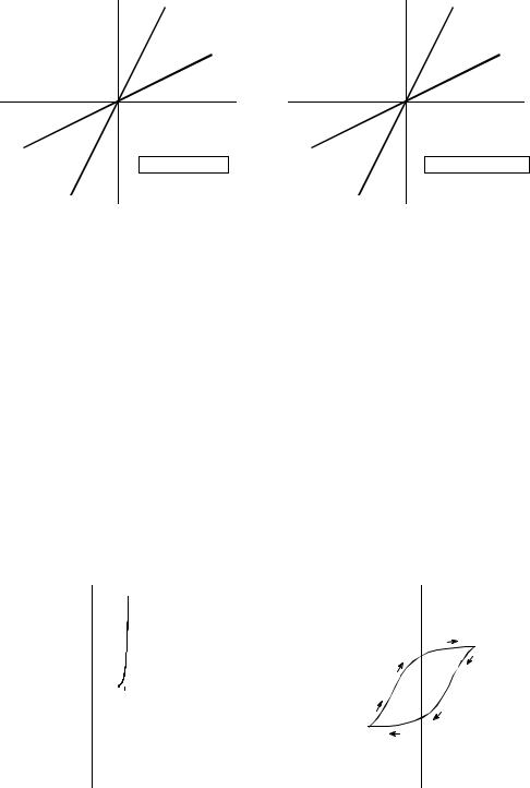
Static linearity defines how a linear system reacts when the signals aren't changing, i.e., when they are DC or static. The static response of a linear system is very simple: the output is the input multiplied by a constant. That is, a graph of the possible input values plotted against the corresponding output values is a straight line that passes through the origin. This is shown in Fig. 5-5 for two common linear systems: Ohm's law for resistors, and Hooke's law for springs. For comparison, Fig. 5-6 shows the static relationship for two nonlinear systems: a pn junction diode, and the magnetic properties of iron.
Chapter 5- Linear Systems |
93 |
Current |
low |
resistance |
|
|
|
|
high |
|
resistance |
|
Voltage |
|
a. Ohm's law |
Elongation |
weak |
|
spring |
||
strong |
||
|
||
|
spring |
|
|
Force |
|
|
b. Hooke's law |
FIGURE 5-5
Two examples of static linearity. In (a), Ohm's law: the current through a resistor is equal to the voltage across the resistor divided by the resistance. In (b), Hooke's law: The elongation of a spring is equal to the applied force multiplied by the spring stiffness coefficient.
All linear systems have the property of static linearity. The opposite is usually true, but not always. There are systems that show static linearity, but are not linear with respect to changing signals. However, a very common class of systems can be completely understood with static linearity alone. In these systems it doesn't matter if the input signal is static or changing. These are called memoryless systems, because the output depends only on the present state of the input, and not on its history. For example, the instantaneous current in a resistor depends only on the instantaneous voltage across it, and not on how the signals came to be the value they are. If a system has static linearity, and is memoryless, then the system must be linear. This provides an important way to understand (and prove) the linearity of these simple systems.
Current |
B |
0.6 v Voltage |
|
H |
a. Silicon diode |
|
b. Iron |
FIGURE 5-6
Two examples of DC nonlinearity. In (a), a silicon diode has an exponential relationship between voltage and current. In (b), the relationship between magnetic intensity, H, and flux density, B, in iron depends on the history of the sample, a behavior called hysteresis.
94 |
The Scientist and Engineer's Guide to Digital Signal Processing |
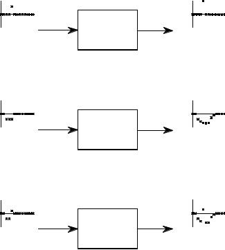
An important characteristic of linear systems is how they behave with sinusoids, a property we will call sinusoidal fidelity: If the input to a linear system is a sinusoidal wave, the output will also be a sinusoidal wave, and at exactly the same frequency as the input. Sinusoids are the only waveform that have this property. For instance, there is no reason to expect that a square wave entering a linear system will produce a square wave on the output. Although a sinusoid on the input guarantees a sinusoid on the output, the two may be different in amplitude and phase. This should be familiar from your knowledge of electronics: a circuit can be described by its frequency response, graphs of how the circuit's gain and phase vary with frequency.
Now for the reverse question: If a system always produces a sinusoidal output in response to a sinusoidal input, is the system guaranteed to be linear? The answer is no, but the exceptions are rare and usually obvious. For example, imagine an evil demon hiding inside a system, with the goal of trying to mislead you. The demon has an oscilloscope to observe the input signal, and a sine wave generator to produce an output signal. When you feed a sine wave into the input, the demon quickly measures the frequency and adjusts his signal generator to produce a corresponding output. Of course, this system is not linear, because it is not additive. To show this, place the sum of two sine waves into the system. The demon can only respond with a single sine wave for the output. This example is not as contrived as you might think; phase lock loops operate in much this way.
To get a better feeling for linearity, think about a technician trying to determine if an electronic device is linear. The technician would attach a sine wave generator to the input of the device, and an oscilloscope to the output. With a sine wave input, the technician would look to see if the output is also a sine wave. For example, the output cannot be clipped on the top or bottom, the top half cannot look different from the bottom half, there must be no distortion where the signal crosses zero, etc. Next, the technician would vary the amplitude of the input and observe the effect on the output signal. If the system is linear, the amplitude of the output must track the amplitude of the input. Lastly, the technician would vary the input signal's frequency, and verify that the output signal's frequency changes accordingly. As the frequency is changed, there will likely be amplitude and phase changes seen in the output, but these are perfectly permissible in a linear system. At some frequencies, the output may even be zero, that is, a sinusoid with zero amplitude. If the technician sees all these things, he will conclude that the system is linear. While this conclusion is not a rigorous mathematical proof, the level of confidence is justifiably high.
Examples of Linear and Nonlinear Systems
Table 5-1 provides examples of common linear and nonlinear systems. As you go through the lists, keep in mind the mathematician's view of linearity (homogeneity, additivity, and shift invariance), as well as the informal way most scientists and engineers use (static linearity and sinusoidal fidelity).
Chapter 5- Linear Systems |
95 |
Examples of Linear Systems
Wave propagation such as sound and electromagnetic waves
Electrical circuits composed of resistors, capacitors, and inductors
Electronic circuits, such as amplifiers and filters
Mechanical motion from the interaction of masses, springs, and dashpots (dampeners)
Systems described by differential equations such as resistor-capacitor-inductor networks
Multiplication by a constant, that is, amplification or attenuation of the signal
Signal changes, such as echoes, resonances, and image blurring
The unity system where the output is always equal to the input
The null system where the output is always equal to the zero, regardless of the input
Differentiation and integration, and the analogous operations of first difference and running sum for discrete signals
Small perturbations in an otherwise nonlinear system, for instance, a small signal being amplified by a properly biased transistor
Convolution, a mathematical operation where each value in the output is expressed as the sum of values in the input multiplied by a set of weighing coefficients.
Recursion, a technique similar to convolution, except previously calculated values in the output are used in addition to values from the input
Examples of Nonlinear Systems
Systems that do not have static linearity, for instance, the voltage and power in a resistor: P ' V 2R , the radiant energy emission of a hot object depending on its temperature: R ' kT 4 , the intensity of light transmitted through a thickness of translucent material: I ' e & "T , etc.
Systems that do not have sinusoidal fidelity, such as electronics circuits for: peak detection, squaring, sine wave to square wave conversion, frequency doubling, etc.
Common electronic distortion, such as clipping, crossover distortion and slewing
Multiplication of one signal by another signal, such as in amplitude modulation and automatic gain controls
Hysteresis phenomena, such as magnetic flux density versus magnetic intensity in iron, or mechanical stress versus strain in vulcanized rubber
Saturation, such as electronic amplifiers and transformers driven too hard
Systems with a threshold, for example, digital logic gates, or seismic vibrations that are strong enough to pulverize the intervening rock
Table 5-1
Examples of linear and nonlinear systems. Formally, linear systems are defined by the properties of homogeneity, additivity, and shift invariance. Informally, most scientists and engineers think of linear systems in terms of static linearity and sinusoidal fidelity.
96 |
The Scientist and Engineer's Guide to Digital Signal Processing |
Special Properties of Linearity
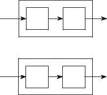
Linearity is commutative, a property involving the combination of two or more systems. Figure 5-10 shows the general idea. Imagine two systems combined in a cascade, that is, the output of one system is the input to the next. If each system is linear, then the overall combination will also be linear. The commutative property states that the order of the systems in the cascade can be rearranged without affecting the characteristics of the overall combination. You probably have used this principle in electronic circuits. For example, imagine a circuit composed of two stages, one for amplification, and one for filtering. Which is best, amplify and then filter, or filter and then amplify? If both stages are linear, the order doesn't make any difference and the overall result is the same. Keep in mind that actual electronics has nonlinear effects that may make the order important, for instance: interference, DC offsets, internal noise, slew rate distortion, etc.
FIGURE 5-7
The commutative property for linear systems. When two or more linear systems are arranged in a cascade, the order of the systems does not affect the characteristics of the overall combination.
IF
x[n] |
System |
System |
y[n] |
|
A |
B |
|
THEN |
|
|
|
x[n] |
System |
System |
y[n] |
|
B |
A |
|
Figure 5-8 shows the next step in linear system theory: multiple inputs and outputs. A system with multiple inputs and/or outputs will be linear if it is composed of linear subsystems and additions of signals. The complexity does not matter, only that nothing nonlinear is allowed inside of the system.
To understand what linearity means for systems with multiple inputs and/or outputs, consider the following thought experiment. Start by placing a signal on one input while the other inputs are held at zero. This will cause the multiple outputs to respond with some pattern of signals. Next, repeat the procedure by placing another signal on a different input. Just as before, keep all of the other inputs at zero. This second input signal will result in another pattern of signals appearing on the multiple outputs. To finish the experiment, place both signals on their respective inputs simultaneously. The signals appearing on the outputs will simply be the superposition (sum) of the output signals produced when the input signals were applied separately.